Diagnostic Equipment:
How can we understand better what our air rifles are doing?
Spring piston air rifles are deceptively simple. They “just” use a spring to drive a piston down a compression chamber and that compressed air drives a pellet out of the barrel and towards the target.
However, in the roughly 10 milliseconds (ms) it takes for the pellet to leave the barrel, the air in the compression chamber reaches over of 1,200 °F and 900 PSI when the piston reaches about 95% of its stroke (adiabatic compression), the rifle recoils back, but then starts to move forward as the piston stops its forward motion and bounces backward. To understand what is going on involves mechanics (spring energy, kinetic energy, friction, etc.) as well as thermodynamics of a compressible fluid. This is what makes spring piston air rifles so fascinating, fun and, at times, frustrating!
In an effort to better understand what is going on with spring piston air rifles, Hector Medina suggested that we work together on some basic tests of three spring piston air rifles (Walther LGU, Walther LGV, and a FWB 124). I have really enjoyed working with him on this journey and we are also grateful to Willem Laan for his support and helpful questions and suggestions. Since many discoveries begin with good questions, the chapter titles are simple questions. We began with just a few questions, but as you will see, the number of chapters grew to NINE!
So let’s take a closer look at how we can use various diagnostic tools to better understand our air rifles.
The simplest, and probably the most important tool, consists of a piece of paper with an aiming point drawn on it! In the end, the most important criterion for any air rifle is how well it can place its shots on a target. Lots of power is useless without accuracy. The famous gun writer Col. Townsend Whelen once said that “Only accurate rifles are interesting.” So you’ll see lots of shots on targets in these blog entries and I hope that you’ll find the rifles that we tested “interesting.” But the targets don’t always tell you why a rifle is shooting well or poorly, so we need to use other diagnostic tools.
Chronograph
One of the first diagnostic tools that is readily available is a chronograph, which gives the muzzle velocity of the pellet. By placing the chronograph at different distances from the muzzle one also can determine how quickly the pellet is slowing down, which gives us the ballistic coefficient (BC) of the pellet-rifle combination. The BC lets us model the trajectory of the pellet better and tells us how well the pellet handles wind; high BC pellets do much better than low BC pellets in windy conditions. Commercial chronographs are available for under $100 (be sure to get LED lights for indoor shooting) or you can make your own for a few dollars, as I did. I used scrap wood and wire and only had to spend a few bucks on infrared LEDs and photodiodes. The Softchrono app (the software can be downloaded here), which was originally designed to use the sound of the rifle firing and the pellet hitting the target to obtain muzzle velocity can be easily adapted to use the signals from the LED/photodiode light gates going into a computer’s audio jack to measure pellet velocity. The nice thing about using infrared LEDs and photodiodes in this DIY chronograph is that one doesn’t have to worry about visible light coming from different places messing up the light gate signals. For more details, please see this thread (my chrono is described in post #6):
https://www.tapatalk.com/groups/yellow/viewtopic.php?p=1899493#p1899493
For the original Poor Man's Electronic Chronograph post, with more details on the audio jack circuit, as well as the infrared LEDs and photodiodes, please check:
https://www.tapatalk.com/groups/yellow/poor-man-s-electronic-chronograph-t186868.html
A chronograph is especially important in spring piston air rifles, because the muzzle velocity (and especially changes in MV) can be a symptom of bad seals, poor/old lubrication, weakening mainspring, poor/irregular fit of pellets in bore, dirty bore, etc.
Recoiloscope
One of the most critical aspects of spring piston air rifles is that the pellet’s point of impact (POI) depends much more on how the rifle is held than for most kinds of other rifles (pneumatic air rifles and powder burners). This is called hold sensitivity, and a good way to study this is to see how the air rifle moves at firing. To measure the rifle’s backward/forward motion on firing, I’ve borrowed an excellent recoil sled that was designed and built by Steve Herr (aka Nitrocrushr on GTA), who was kind enough to send us these photos and diagram.
One of the most critical aspects of spring piston air rifles is that the pellet’s point of impact (POI) depends much more on how the rifle is held than for most kinds of other rifles (pneumatic air rifles and powder burners). This is called hold sensitivity, and a good way to study this is to see how the air rifle moves at firing. To measure the rifle’s backward/forward motion on firing, I’ve borrowed an excellent recoil sled that was designed and built by Steve Herr (aka Nitrocrushr on GTA), who was kind enough to send us these photos and diagram.
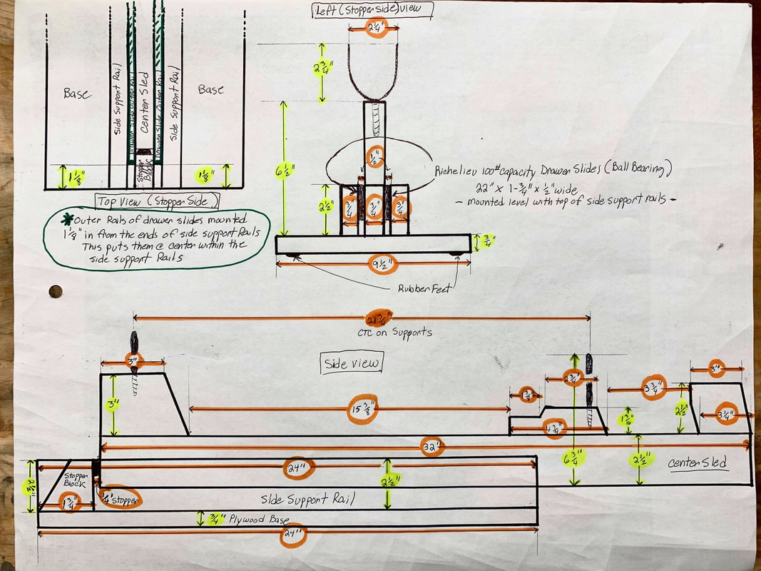
Fig. 1.1 Dimensioned build diagram of Steve Herr’s recoil sled.
Figure 1.2 shows a photo of an air rifle mounted on the sled. The rifle is supported on the sled by u-shaped vinyl-coated hooks (labelled 1 in Fig 1.2) under the forearm and under the stock near the buttplate. A long hook and loop strap (labelled 2 in Fig 1.2) is wrapped around the pistol grip or through the back of the trigger guard to pull the rifle tight against a vertical stop at the back of the sled. The sled itself is held onto the base by ball-bearing drawer slides. There is very little friction in moving the sled back and forth. A ruler (labelled 3 in Fig 1.2) is placed on the base next to the sled to measure sled position. Bubble levels (labelled 4 in Fig 1.2) make sure that the sled is level side-to-side and front-to-back. Finally an air bladder (labelled 5 in Fig 1.2) from a blood pressure cuff is used to depress trigger without moving the rifle. Very clever idea Steve!
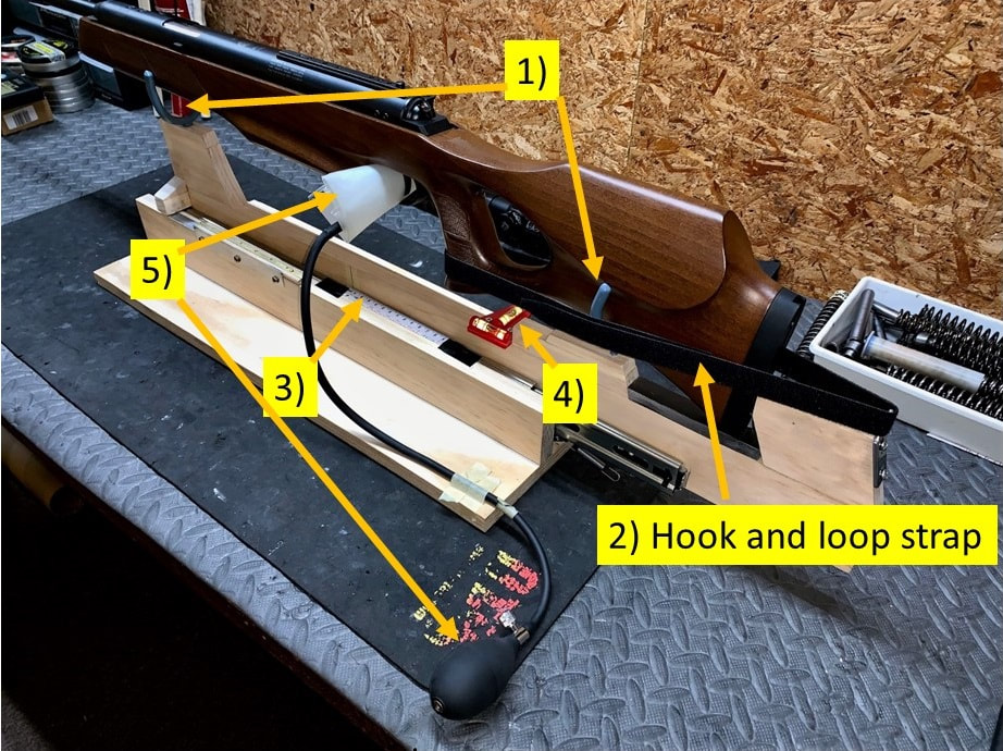
Fig. 1.2 Steve Herr’s recoil sled with rifle attached. Also visible are 1) u-shaped supports, 2) hook and loop strap, 3) ruler to measure sled position, 4) bubble levels and 5) air bladder to depress trigger without moving the rifle.
For more info on the sled, please see:
https://www.gatewaytoairguns.org/GTA/index.php?topic=160511.msg155787786#msg155787786
Figure 1.3 shows how I used the sled to make recoil measurements. For the short distances travelled (~6mm=0.25”) and the short times (10's of milliseconds), the friction of the sled has a negligible impact on the energy and momentum of the recoiling rifle. In fact, one probably could get away with just resting the rifle on sandbags, but the sled makes the recoil measurements much easier, more repeatable, and more accurate. One complication that the sled adds is that the sled itself, which moves with the rifle, weighs 2.4 lbs. This added weight to the rifle will affect its recoil a bit.
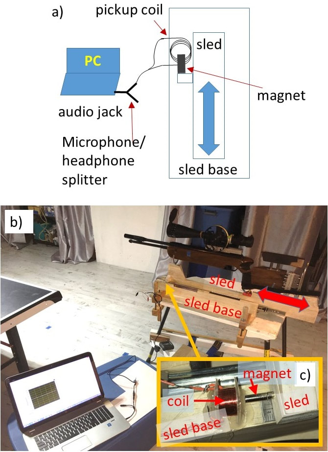
Fig. 1.3 Our recoiloscope: Recoil trace measurement using a the sound card on laptop PC. a) setup schematic, b) setup photo, and c) close-up photo of magnet and coil. The magnet moves with the sled as rifle recoils and the coil is stationary on the sled base.
So what do we measure with the sled? The first thing one can do is take a video of the recoiling rifle. Steve placed an indicator on the sled that points to the ruler on the sled base, so one can see the position of the sled as a function of time. Most smartphones have a high speed video setting with a frame rate of 240 frames per second. This gives a time resolution of just over 4 ms that can capture the recoil motion reasonably well.
Below are some videos that I took of the LGV, LGU, and FWB 124 fired on Steve’s sled.
Make sure you select the lowest play-back speed (0.25X).
LGV recoil video:
https://youtu.be/rh9VVykKKiM
LGU recoil video:
https://youtu.be/ynzrbddtN1U
FWB 124 recoil video:
https://youtu.be/2RKUY3x48zE
These videos give a good qualitative picture of how the rifle is recoiling and one can clearly see the forward surge after the initial backwards recoil, as well as the later oscillations. However, the poor time and spatial resolution make it hard to study the recoil in detail. To get more accurate sled position data with better time resolution, I built an inductive pickup coil system that measures the velocity of the sled with respect to the sled base. As can be seen in the diagram in Fig. 1.3a), I attached a permanent magnet (neodymium-iron- boron rare earth magnet) to the sled that moves with respect to a wire coil that is attached to the sled base. The motion of the magnet with respect to the base produces a voltage in the coil that can be recorded as a function of time with an oscilloscope. In this case I used a soundcard on my laptop computer to record the signal (pc oscilloscope) and later we’ll use some stand-alone oscilloscopes. The voltage is proportional to the velocity of the magnet, so we can measure the rifle/sled velocity during recoil with a sub-millisecond time resolution. A photo of the system is shown in Fig. 1.3b) and a close-up photo of the magnet/pickup coil is shown in Fig. 1.3c).
The basic physical principle that allows this system to measure the sled velocity is Faraday’s law of induction, which basically says that an electrical current will be induced in a coil of wire if the magnetic field, going through the area bound by that coil, changes. As the sled moves back and the permanent magnet moves away from the coil, the amount of magnetic field going through the coil decreases, and a voltage will be induced in the coil that produces an electrical current to try to replace that lost magnetic field.
Electrical currents in coils produce magnetic fields, so the induced currents can actually replace some of the lost magnetic field as the permanent magnet moves away from the coil. The change in magnetic field at the coil is directly proportional to how fast the magnet is moving away from, or towards, the coil, so the coil voltage is proportional to the velocity of the magnet/sled. I made the coil by winding exceptionally fine magnet wire (OD about 0.002”) around a sewing machine bobbin (I did get permission from my wife to steal one of her bobbins!). I mounted the bobbin on a dowel, which I then spun on a power drill. I lost track of the number of turns after about 100, and went until the wire broke. I got roughly the first third of the bobbin wound with wire. The more turns of wire in the coil, the more sensitive the system will be.
Since the system allows one to see the rifle’s recoil and since the signal is picked up with an oscilloscope, we like to call it the “recoiloscope.” A schematic of the recoiloscope is shown in Fig. 1.3a). One can use the audio jack on a computer and oscilloscope software to read the coil voltage (and thereby the sled velocity) as a function of time. I wrote my own data-taking program using National Instrument’s LabView, but there are lots of sound card oscilloscope programs that you could use. I’ve also used Soundcard Scope (https://www.zeitnitz.eu/scope_en), which is free but unfortunately doesn’t allow you to save the data.
Figure 1.3b) shows a photo of the setup, including the customized Walther LGU that was used for all the tests in this chapter. More info on the rifle can be found at:
https://www.gatewaytoairguns.org/GTA/index.php?topic=168525.0
It’s important to mention that this system was inspired by Jim Tyler, who developed an electrical “recoilometer.” His monthly Technical Airgun column in Airgun World magazine is brilliant and full of deep insights into the finer inner workings of spring piston airguns. Although Jim does not give much technical detail on his recoilometer, I’m assuming it operates using a pick-up coil system as well.
Figure 1.4 shows a typical recoil trace from a Walther LGU measured using the recoiloscope from Fig. 1.3. The vertical axis in the plot in Fig. 1.4 is the coil voltage, which is proportional to the sled/rifle velocity, and the horizontal axis is time in seconds. Positive voltages correspond to the rifle moving forward and negative voltages mean the rifle is moving backward.
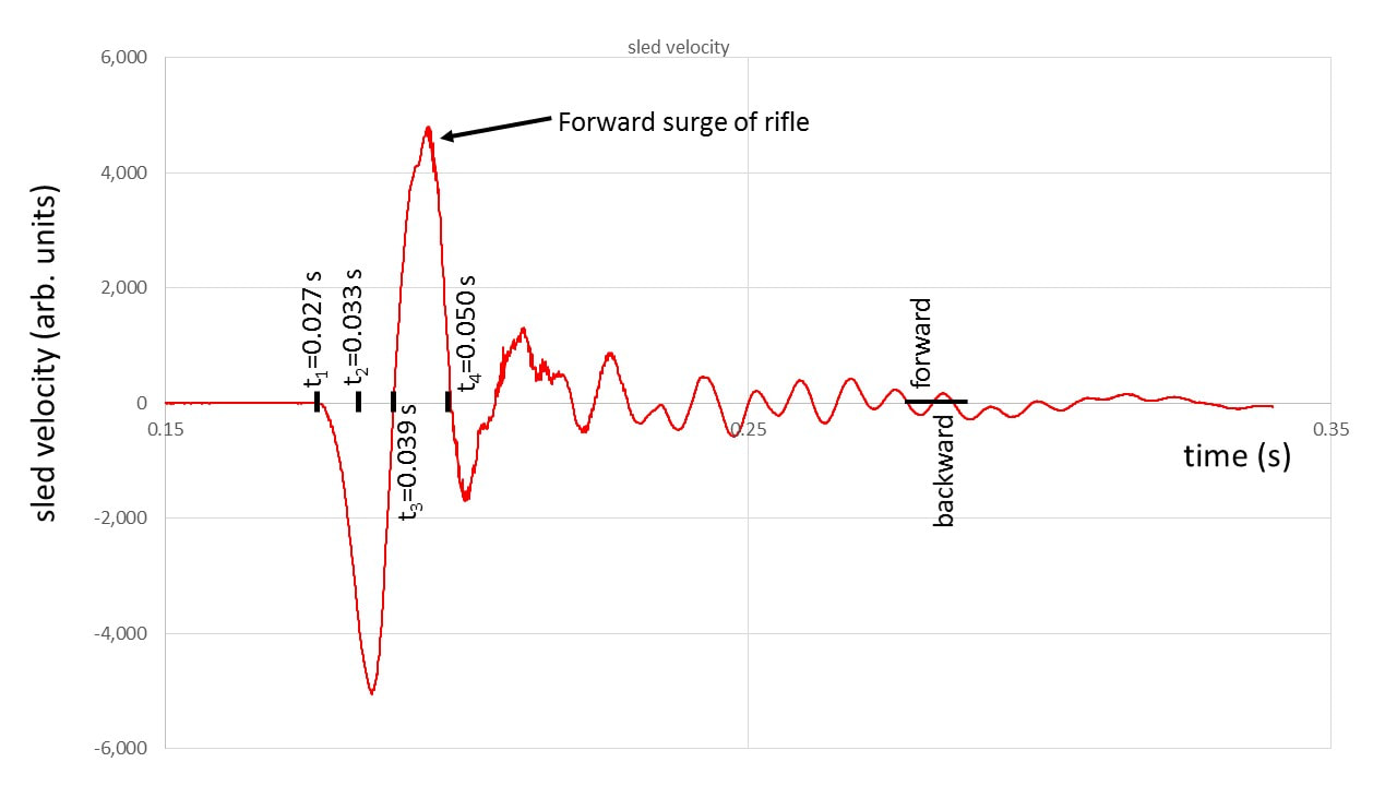
Fig. 1.4 Recoil trace using the recoiloscope with a laptop PC. t1 is when the rifle starts recoiling backwards. t2 is when the rifle reaches the maximum rearward velocity and starts slowing down it rearward motion. t3 is when the rifles starts to surge forward. t4 is when the rifle starts going backward again and begins smaller oscillations backward and forward.
Unlike a firearm, where the recoil is strictly backward, a spring piston airgun exhibits a strong forward surge as the piston slows down/stops at the front end of its travel. One way to think of it is that the rifle must apply a backwards force to the piston to stop it, and therefore, by Newton’s third law, the piston must be pushing the rifle forward with the same magnitude force.
In Fig. 1.4, several key times are identified. When the trigger is pulled and the piston accelerates forward, the rifle starts to recoil backward at time t1. About 6 ms later, at time t2, the rifle reaches the maximum rearward velocity and starts slowing down its rearward motion. It’s still going backwards, but is slowing down. At time t3, 12 ms after the start of the recoil, the piston slows down and the rifle starts to surge forward. At time t4, 23 ms after the start of the recoil, rifle recoils backward again and begins smaller oscillations backward and forward. I think that these smaller oscillations are caused by coils in the mainspring vibrating back and forth.
In Fig. 1.4, several key times are identified. When the trigger is pulled and the piston accelerates forward, the rifle starts to recoil backward at time t1. About 6 ms later, at time t2, the rifle reaches the maximum rearward velocity and starts slowing down its rearward motion. It’s still going backwards, but is slowing down. At time t3, 12 ms after the start of the recoil, the piston slows down and the rifle starts to surge forward. At time t4, 23 ms after the start of the recoil, rifle recoils backward again and begins smaller oscillations backward and forward. I think that these smaller oscillations are caused by coils in the mainspring vibrating back and forth.
Dynamograph
Since the pellet is disturbed by the motion of the rifle only while the pellet is in the barrel, a key question is:
When does the pellet leave the barrel? To measure the pellet exit time, I combined the recoiloscope with the homemade chronograph that I mentioned earlier in this chapter. We call this system a “dynamograph.”
The DIY chronograph requires a laptop pc (to power the infrared LEDs and the light gate circuit). I borrowed a two-channel digital storage scope (Tektronix TDS 2024B) to simultaneously measure the pickup coil signal (sled velocity) and the light gate signal (when pellet crosses under the light gates in the DIY chronograph). The oscilloscope doesn’t have to be anything special. The main features are that it can record two channels at the same time, has a time resolution of 0.1 ms or faster, and can save the data so that we can analyze and plot the traces. As we’ll see later, it’s helpful to have an oscilloscope that can do dc as well as ac input coupling. At the end of the discussion of the dynamograph, I will test a $100 mini USB oscilloscope and show that it can work as well as the Tektronix oscilloscope.
Figure 1.5a) shows a schematic of the dynamograph. The recoil velocity measurement is the same as before except that now the pickup coil signal goes to channel 1 of the oscilloscope instead of the sound card on a PC. The oscilloscope measures the pickup coil voltage, which tells us about the sled velocity, and the light gate signal from the DIY chronograph, which tells when the pellet crosses the light gates in front of the muzzle. The PC now only serves to power the LEDs of the light gate through its USB port and to power the photodiode detectors in the light gate circuit through the audio jack port. The pickup coil voltage goes to channel 1 on the oscilloscope and the light gate voltage (two new wires are connected to the original light gate circuit) goes to channel 2. This allows us to record the sled velocity and the pellet crossing the light gates at the same time.
The DIY chronograph is connected to the PC the same way as it was for use as a chronograph except that the two wires (blue wires going to Ch. 2 of oscilloscope in Fig. 1.5a) are connected to the light gate circuit going to the PC’s audio jack (black wires in Fig. 1.5a). One of the wires connects before the first light gate and the other one connects after the second light gate, so we’re measuring the voltage across the entire photodiode circuit. When the pellet goes through a light gate, it blocks the light from the infrared LED at the top of the gate from going to the photodiodes (detectors) at the bottom of the gate, which causes a positive voltage spike in the photodiode circuit.
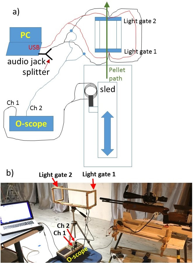
Fig. 1.5 Our dynamograph records the recoil velocity and pellet exit signal using an oscilloscope and DIY chronograph. a) setup schematic and b) setup photo.
As mentioned before, the dynamograph records the velocity of the sled as a function of time on Ch. 1 on the oscilloscope, while on Ch. 2 we can see when the pellet leaves the muzzle, passing light gate 1 and when it passes the second light gate, which is 1.88 ft after the first light gate. The time separation between the light gate pulses gives us the pellet’s velocity, whereas the first light gate pulse gives us the time when the pellet left the barrel, and is no longer affected by rifle vibration/motion. Since LG1 is not exactly at the muzzle but is located about six inches away from it, the LG1 pulse occurs about 0.6 ms after the pellet leaves the barrel (assuming a pellet velocity around 800 fps), but that’s close enough for the time scales that we’re looking at. From now on, we’ll just treat the LG1 pulse as the time the pellet leaves the barrel, but if you wanted to be super accurate, you could subtract 0.6 ms to get the actual time the pellet leaves the muzzle.
Figure 1.5b) shows a photo of the dynamograph setup, again with my trusty LGU. The light gates are labeled in the photo. You can see how the DIY chronograph is connected to the PC (USB port and audio jack), and how the wires from the sled pickup coil go to Ch. 1 on the oscilloscope and the wires from the DIY chronograph go to Ch. 2 on the oscilloscope (labeled “o-scope” in figure).
Figure 1.6b) shows the measured pickup coil voltage (sled velocity) in red in the middle plot. I’m using red for all the velocity plots in this chapter to emphasize that it is a directly measured quantity, within a scaling factor.
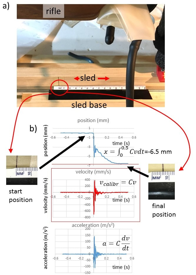
Fig. 1.6 Recoil traces using the dynamograph over 1s. We can measure the final position of the sled using ruler on sled base shown in a). The sled starts at 0.0 mm and ends at -6.5 mm when recoil motion has finished (see photos in b). The sled velocity (red plot in middle graph), position and acceleration are shown in b). Knowing the final position of the sled (red horizontal line in top graph near -6.5 mm in b) allows us to calibrate the velocity and acceleration by determining C.
One important question is: What is the absolute magnitude of the rifle’s velocity? Also: Can we determine the position and acceleration of the rifle?
We could try moving the rifle/sled at a known speed and simply multiply the pickup coil voltage by a calibration factor to produce the actual speed in mm/s, but there’s an easier way. Although measuring velocity is tricky, measuring the starting and ending position of the sled position is very straightforward. Thanks to Newton and Leibnitz, and through a bit of calculus, we know how position, velocity, and acceleration are connected. The velocity is just how fast the position is changing with time, and the acceleration is just how fast the velocity is changing with time. So if we add up all the changes in position with time (integrate the velocity) we can get the position as a function of time. This turns out to be the area under the velocity curve, and if we integrate the velocity from the start time to the time when the sled reaches its final position, we should just get the final position, which we can measure with a ruler (see Fig. 1.6a). The photos in Fig. 1.6b) show the initial and final positions of the sled. This allows us to determine the constant C, by which we have to multiply the pickup coil voltage to get the actual velocity vs time. In Fig. 1.6, I found that multiplying the pickup coil voltage by C=520 produces a final position of around -6.5 mm, which is the final position of the sled that I measured.
For a video on how one can get the position of an object from its velocity history, please check out this video:
ttps://www.khanacademy.org/science/ap-physics-1/ap-one-dimensional-motion/instantaneous-velocity-and- speed/v/why-distance-is-area-under-velocity-time-line
Since acceleration is defined as the rate at which velocity is changing with time, we can determine the acceleration by looking at the slope of the velocity vs time plot, which is the derivative of velocity. So with the dynamograph we can measure the velocity of the rifle/sled as a function of time with sub-ms resolution, and then use that velocity trace to get the position and acceleration of the rifle (through integration and differentiation, respectively), as functions of time.
So, knowing the distance that the rifle has traveled at the end of the recoil cycle allows us to calibrate everything!
One concern about this simple calibration technique is whether the calibration factor is the same for all positions of the sled. For example, the pickup coil signal when the sled is traveling at a constant velocity of 500 mm/s towards the coil may change as the magnet gets closer to the coil. The pattern of magnetic field lines produced by the magnet is complicated and highly non-linear, so maybe the sensitivity of the pickup coil to the motion of the magnet may be different when the magnet is close compared to when it is far away from the coil?
To check this, I moved the sled different distances from the coil at different speeds by hand to obtain a series of velocity vs time plots. Then I integrated the velocity plots to determine the distance traveled in each run and compared that distance with the measured distance traveled in each run.
Figure 1.7 shows a series of runs that always began with the sled in the forward most position at 0.0 mm. I then moved the sled back 3.0, 5.0, 7.0, and 10.0 mm (distance D in Fig. 1.7), recording the pickup coil signal of each run on the oscilloscope. For the 5.0 mm and 10.0 mm runs, I moved the sled at different speeds. You can see clearly that the distance traveled scales with the depth and width of the velocity dip (red curves). It’s also reassuring that although the dips for the slow and fast displacement look different, the areas are the same for the same displacement. The velocity dips for the slow displacements are shallow but wide while the dips for the fast displacements are deep but narrow, so the areas that roughly go as the depth times the width of the dip remain the same. For all distances and speeds, the distance obtained by integrating the pickup coil signal using the same calibration constant was well within 10% of the actual distance by which the sled was moved. I can only measure distances to within about 0.5 mm, so these errors could just be due to the uncertainty in the distance measurements. Since we’re more interested in qualitative behavior, I didn’t think it was worth improving the accuracy of these measurements. Also, since we’re comparing three rifles using the same dynamograph with the same calibration factor, the relative behavior should not be affected by any systematic calibration errors.
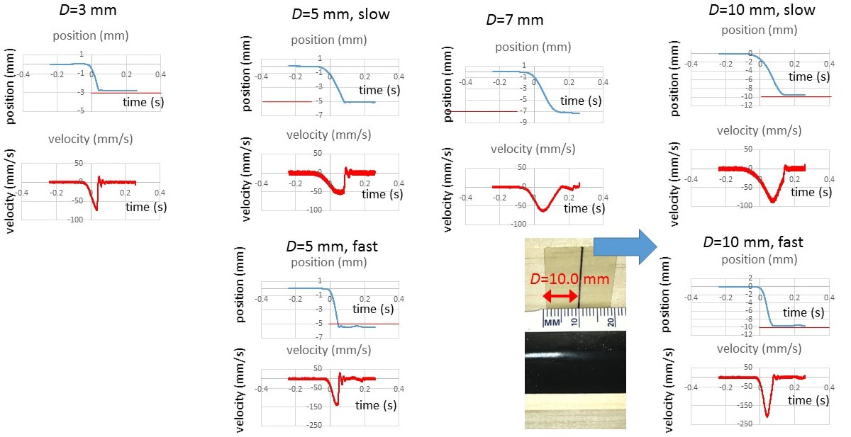
Fig. 1.7 Further calibration testing of the dynamograph. I moved the sled known distances D at different speeds by hand to check the calibration constant C that was obtained in Fig. 1.4. The measured final positions are shown with red horizontal lines. Photo shows D=10.0 mm.
Figure 1.8 shows a closer view of the calibrated position, velocity, and acceleration of the LGU during recoil.
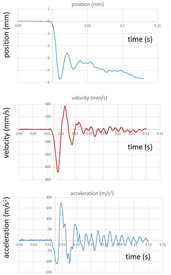
Fig. 1.8 Recoil traces from my LGU using the dynamograph. Position, velocity, and acceleration were calibrated using calibration constant C.
Going through the Motions
Now that we have calibrated our apparatus, the position, velocity, and acceleration have actual units that mean something. As can be seen in Fig. 1.8 above, the maximum velocity of the rifle/sled during the entire recoil process is about 680 mm/s (2.2 fps) to the rear, occurring at time 0.005 s. The maximum acceleration is actually forward at about 165 m/s² (about 17 times the acceleration of gravity, 17 g's). This is not too surprising since the piston accelerates forward more gently at the start of the recoil (and therefore the rifle accelerates backward) but then stops more abruptly near the front end of the stroke, causing the rifle to accelerate forward more dramatically. One can imagine that if I forgot to put a pellet in the barrel, there would be less of a cushion of air to slow the piston down at the end of its forward stroke and it would slam into the front of the compression chamber, producing a huge change in velocity in a very short time and causing the rifle to jump forward with a big acceleration!
The recoil motion of the entire rifle that is shown in Fig. 1.8 can also be used to gain insight into what is going on inside the rifle. One may ask why does the rifle move when fired in the first place? There are two equivalent ways to looks at this.
When the trigger is pulled on a spring piston airgun, the compressed spring is allowed to expand, pushing the piston forward. Newton’s third law states that if a force is applied to an object, that object pushes back on whatever is applying the force with an equal magnitude force in the opposite direction. So the rifle is pushing the piston forward via the mainspring and the piston is therefore pushing back on the rifle, also via the mainspring, with the same magnitude force, but in the opposite direction. Since force is equal to mass times acceleration and the forces on the piston and rifle are the same magnitude, the heavier rifle will accelerate backward with a smaller acceleration than the lighter piston accelerates forward.
Another way to look at this is through conservation of momentum. The momentum of an object is simply the mass of that object times its velocity. In a system where there are no external forces, the total momentum of all the parts of that system remains constant. In this case, our system consists of the rifle/sled without the piston (which I’ll just call “rifle” in this paragraph) and the piston. The dominant forces here are the rifle pushing on the piston and the piston pushing back. The weak external force of friction in the sliding sled that acts against the motion of the system (rifle + piston) can be neglected. In this case the total momentum of the rifle and piston is zero before the shot is fired, neither is moving. After firing, the total momentum should still remain zero at all times and the forward momentum (positive velocity) of the piston is exactly cancelled by the rearward momentum (negative velocity) of the recoiling rifle. Using momentum conservation and assuming that the dominant moving part in the air rifle is the piston, one can determine the velocity of the piston from the velocity of the rifle itself. For example, in Fig. 1.6 we saw that the air rifle reaches a maximum rearward velocity of -680 mm/s at time 0.005 s. Using conservation of momentum, one can calculate that the velocity of the piston at that same time is around 72.2 fps in the forward direction. Here we neglected the mass of the spring (or parts of the spring) that are moving and just look at the mass of the piston (0.56 lbs) and the mass of the rifle without the piston (15.7 lbs for rifle and 2.4 lbs for the sled produce a total weight of 18.1 lbs), which always move in opposite directions. Unlike a firearm, where the rifle recoils strictly backward due to the forward momentum of the bullet and powder/gas moving forward, for an air rifle one can neglect the momentum of the pellet, which in this case is around 40 times smaller than the momentum of the piston or rifle. The spring is more complicated since it doesn’t move as a single unit. In principle, some coils of the spring could be moving forward while other parts of the spring are moving backward. Luckily the spring is fairly light (0.30 lbs), so neglecting it should not affect our analysis significantly.
One can also use conservation of momentum to estimate how far forward the piston has travelled when it bounces back (and the rifle surges forward). The rifle has moved back around 4.5 mm when the piston bounces back, which suggests (using conservation of momentum) that the piston has moved forward around 14.5 cm. Since the length of the compression chamber ahead of the piston is only around 13 cm, this estimate is clearly not correct! The piston has not gone 1.5 cm past the front end of the compression tube! I think the reason for the overestimate is that I neglected the spring dynamics. Adding just half the spring mass to the piston mass moving forward, reduces the piston stroke to 11.4 cm before it bounces. Unfortunately, we just don’t have enough information to get an accurate estimate of where (although we know when) the piston bounces. This is something that I would like to figure out someday. If we knew where the piston bounces, we would know the volume of the compressed air inside the compression chamber at that time. One can reasonably model air as an ideal gas in this situation and since the compression happens very fast (less than 10 ms), it’s safe to assume that the heat in the gas is trapped and has no time to get transferred to the compression chamber walls. This is called an adiabatic compression and if we know the change in volume, we could also get the change in temperature and pressure of the air in the compression chamber. For a 90% compression, the air pressure would go up to 317 psi and air temperature to over 841 °F. For a 95% compression, the pressure would go up to 904 psi and temperature to over 1294 °F.
The dynamograph not only gives us the calibrated position, velocity and acceleration of the rifle, it also tells us when the pellet left the barrel and how fast it was going.
Figure 1.9 shows both the calibrated rifle velocity (red plot in middle graph) and light gate voltage (orange plot in middle graph). Note that we zoomed in on the time base with a much shorter time range. With the longer time ranges in Figs. 1.6 and 1.8, it’s much harder to catch the short pulses coming from the light gates. Also, we’re mainly interested in what happens before the pellet exits the barrel, since any motion of the rifle after that will not affect the accuracy of the rifle. The two spikes in the orange plot at 0.00768 s and 0.0101 s corresponds to the times when the pellet passed LG1 and LG2, respectively. So now we know that the pellet left the barrel a little before 0.0768 s, when the rifle was still moving backward but was slowing down. This time also happens to be the peak of the forward acceleration, so it probably coincides with the time when the piston is slowing down its forward motion the most abruptly. Since LG1 and LG2 are 1.88 ft apart, we also can determine the muzzle velocity of the pellet to be (1.88 ft)/(0.0101 s- 0.00768 s)=777 fps, which agrees well with separate muzzle velocity measurements that I made with my Caldwell chronograph.
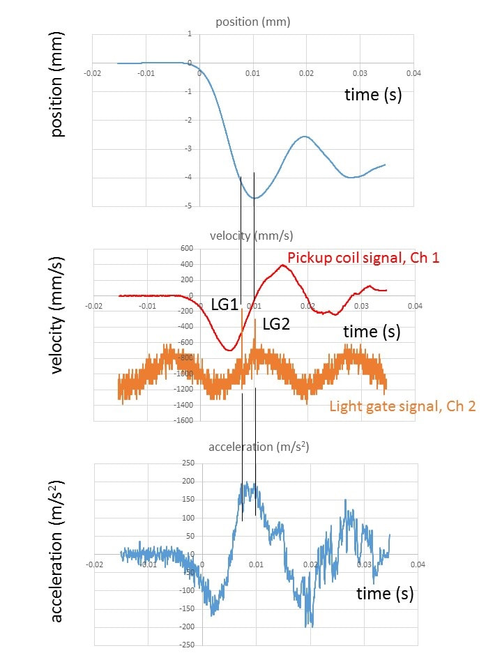
Fig. 1.9 Dynamograph traces showing recoil and pellet exit traces over a shorter time range for my LGU. The pellet crossing the two light gates (LG1 and LG2) can be seen by the two sharp upward spikes in the orange plot in the middle graph. The vertical black lines allow us to see what the recoil is doing at those times. The first light gate (LG1) pulse is when the pellet has travelled a couple of inches in front of the muzzle.
In addition to allowing two signals to be measured at once, the oscilloscope offers another important advantage over using a pc sound card to capture the recoil signal. PC sound cards respond to frequencies ranging from about 10 Hz to over 20 kHz, which means that they can detect changes in signals that are faster than 100 ms but slower than 0.05 ms. Therefore, PC sound cards are more than fast enough to record the air rifle’s recoil signal from the pickup coil. However, any slower motion that is on the order of tenths of a second will not be recorded. There are good reasons why sound cards do not detect such slower signals. First of all, slower signals would cause a drift in the background on top of which the higher frequency audio signals that we want to hear are superimposed. These slow drifts could overload the sound card and cause distortion. Furthermore, since the human ear can’t hear such low frequencies, it makes sense to filter them out before reading them with the sound card. This type of filtering is called ac (alternating current) coupling, which simply means that slow, dc (direct current) signals are filtered out. For fast signals that happen on time scales shorter than 0.1s, both ac- and dc-coupling give the same result. In dynamograph traces most of the action happens pretty fast, on the order of ms. However, there is a slower component that takes a few tenths of a second as the rifle gradually drifts backward to settle to a position around -6.5 mm, as can be seen at the top of Fig. 1.6. This slow behavior will not be picked up by the ac-coupled sound card. A nice feature of most oscilloscopes is that their inputs can be easily switched from ac- to dc-coupling. To test this, I recorded three shots from my LGU, once using dc-coupling on an oscilloscope, once using ac-coupling on an oscilloscope, and once using a computer sound card. The results of these measurements are shown in Fig. 1.10 below.
As you can see, the dc-coupling could follow the slow backward drift of the rifle position, circled in red in Fig.
1.10 a). On the other hand, using ac-coupling in the oscilloscope input and the sound card (which is wired to always be ac-coupled), filtered this drift out and the apparent rifle position returned to zero, as can be seen by the circled regions in Fig. 1.10 b) and c). The fast oscillations look pretty much the same, but to see the slow backward drift, one needs dc-coupling. So if you use a computer sound card, or any other voltage recorder that is ac-coupled, you will not be able to see the slower backward drift of the rifle (which is really there!) and you will not be able to use the final rifle position to calibrate the velocity signal.
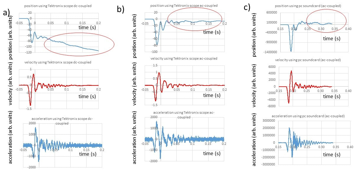
Fig. 1.10 ac vs dc coupling of recoil signals from my LGU. a) oscilloscope with dc coupling, b) oscilloscope with ac coupling, and c) PC soundcard (ac-coupled). The main difference is that the ac-coupling does not show the slower rearward displacement of sled circled in red in the top plots.
I’m ending this section with a test of a mini-USB oscilloscope that Hector found. The DS212 mini-oscilloscope is smaller than a typical smartphone and works quite well!
https://www.sainsmart.com/collections/tools-instruments/products/dso202-2-ch-handheld-mini-digital-oscilloscope-touchscreen
The photo in Fig. 1.11a) shows the Tektronix and DS212 oscilloscopes measuring the pickup coil signal at the same time. You can see how much smaller the DS212 is compared to the Tektronix oscilloscope. The hardest part in using the DS212 was finding a mini usb cable that actually could transfer data to my pc (most of my cables were only for charging). The mini oscilloscope samples 25 points per division (I had to deduce this myself since the manual is pretty sparse, especially when it comes to transferring the data to a pc), so it was easy to scale the time and voltage axes. Figure 1.11b) shows the recoil traces taken simultaneously by the Tektronix and DS212 oscilloscopes. The traces are pretty much right on top of each other. There were no fudge factors and I just had to shift the time scale of the DS212 mini-oscilloscope traces so that they would lie on top of the Tektronix traces. I also used the mini oscilloscope as a dynamograph in Fig. 1.11c). The DS212 is around $100, so it provides a compact and relatively inexpensive alternative to a more expensive benchtop oscilloscope, and we HOPE this accessibility will open the avenue for other researchers to follow the methodology.
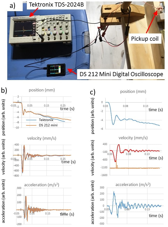
Fig. 1.11 Testing a mini oscilloscope. a) photo of regular and mini oscilloscopes measuring the pickup coil signal at the same time from the LGU, b) recoil traces from the two oscilloscopes, and c) recoil traces and light gate signal using the mini oscilloscope.
What about Efficiency?
The final part of this chapter looks at the efficiency of the spring piston powerplant.
One of the most remarkable aspects of spring piston airguns is that they generate their own power to propel pellets. The kinetic energy that goes into the pellet is easy to measure using a chronograph. The pellet kinetic energy as the pellet leaves the muzzle, commonly known as the muzzle energy (ME) is just ME=v*v*m/2 , where m is the pellet mass and v is its speed. If you’re using mass in grains and velocity in fps, the energy in ft-lbs is: (energy in ft-lbs)= 2.22*10^-6 * (mass in grains)*(velocity in fps)².
The efficiency of an air rifle is simply the muzzle energy of the pellet divided by the work that we put into the rifle by cocking it. To determine the work that we put into an object, we need to measure the applied force F on said object that moved it a distance d. If the object is moving in a straight line with a constant force, work is just F*d. If the magnitude of the force varies as one moves an object along the x-direction, we have to break up the path into smaller pieces, each with length dx, so that the force F(x) within a length dx at position x is roughly constant. Then we just add the bit of work done during each little piece of the path F(x)dx to get the total work (i.e., we integrate).
In some ways, the relations between work, force and distance is the same as the relation between distance, velocity and time. In the explanation above for how we obtain distance from the measurement of velocity that the dynamograph gives us, we explained with the Khan Academy video that showed how the area under the curve of one function equals another function so, in the same way that integrating the velocity over time gives us the distance, integrating the force over the distance gives us the work which, in essence, is the energy we are putting into the rifle.
When cocking an air rifle, we don't really push with a force (F) an object along a distance (d), we apply a torque τ (force at a distance from the pivot -r- that causes rotation) to rotate a barrel or cocking lever by an angle (Θ). If the force F causing the rotation is perpendicular to a line of length r connecting the point where the force applied to the pivot point, then the torque is r*F, where r is the distance from the pivot to the point where the force is applied. If torque were constant, the work W done by the torque to rotate a barrel from a starting angle of Θinitial to a final angle of Θfinal would simply be:
W=τ*( Θfinal - Θinitial )
However, in most air rifles the cocking torque is not constant so we have to add up (integrate) the pieces of work using:
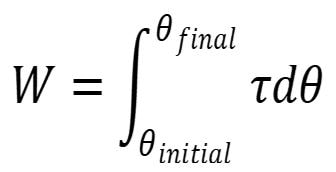
As shown Fig. 1.12a), I clamped the rifle upside down in a padded vise and pulled the barrel with a digital luggage scale. I tried to always keep the pulling force perpendicular to the barrel (otherwise, some of that force would be pushing/pulling along the barrel axis and not causing rotation). Since we need to measure the torque as a function of angle, I used a "Wixey" digital angle gauge attached to the barrel to keep track of its orientation. I loosened the barrel tension screw to reduce the friction in the pivot. I noticed a clear reduction in the force required to keep the barrel at a certain angle when I stopped rotating the barrel. This is due to the fact that static friction holding an object in place is typically higher than kinetic friction, which occurs while the object is moving. The static friction helped keep the barrel in place, thereby reducing the force that I needed to apply. The static friction was fairly large and not very repeatable, so I decided to do the torque measurements in a continuous swing without stopping. Keeping track of the force applied and the barrel’s angle as I rotated the barrel was challenging, so I used a video camera to record the barrel angle reading on the digital angle gauge as well as my voice as I read the force values on the luggage scale as the barrel rotated continuously without stopping, as shown in Fig. 1.12. I then looked at the video using Windows Movie Maker, as shown in Fig. 1.12b). Movie Maker has an audio amplitude trace at the bottom of the video, so I could easily find the places (peaks in the audio trace) where I read out the luggage scale reading. At each of these places, I could then read the digital angle scale in the video and obtain torque as a function of angle.
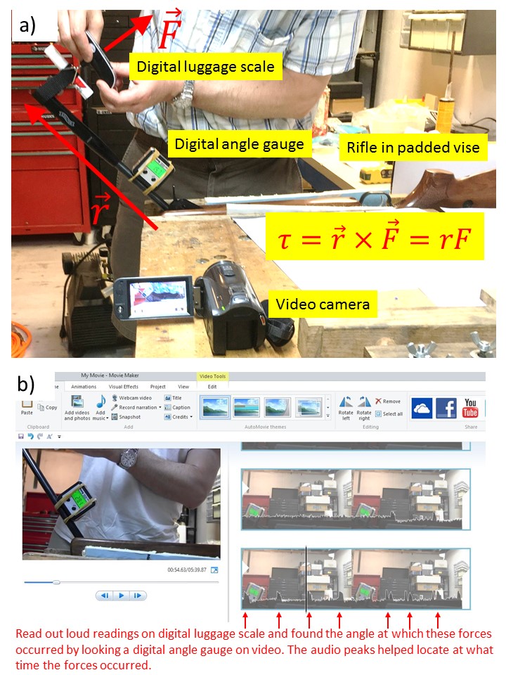
Fig. 1.12 Cocking work measurement. a) setup photo and b) video still during measurement.
Figure 1.13 shows the total torque as a function of angle (blue symbols) that I measured for a Walther LGV. In
order to subtract the background torque coming from pivot friction and other sources, I repeated measurement with the rifle already cocked (orange plot in Fig. 1.13). Initially, one has to lift the barrel up as it rotates, so there’s some background torque due to the weight of the barrel itself! By subtracting the background torque, one can get closer to the actual work that one is putting into the mainspring itself.
Unfortunately, this subtraction technique does not eliminate the work that arises from going against the piston seal friction as the piston moves back during cocking. To get a more accurate torque background measurement, one should completely remove the spring, which would allow the friction in the piston seal to be included in the background work. If one is interested in efficiency in terms of how much work the shooter has to do in using the rifle, then all these sources of friction should be included. What I’m trying to isolate here is how much of the energy in the spring gets transferred to the pellet, so I’m removing any wasted work in cocking the rifle that doesn’t go into the spring. As you can see, the torque increases as the barrel pivots, but the ends of the plot are a bit flattened. The s-shaped curve makes sense as the large mechanical advantage at the beginning and end of the cocking stroke tends to compensate the increasing force required to compress the spring. I used a 4th order polynomial to fit the torque vs angle, and then integrated (see equations at the bottom of Fig 1.13). The data are pretty reproducible and the fit looks good. For this particular run, the total cocking work was 35.4 ft-lbs and the background friction/barrel weight work was 2.0 ft-lbs, which means that 33.4 ft-lbs of energy went into the spring. The typical pellet muzzle energy for this rifle is around, 12.4 ft-lbs, which gives us an efficiency of around 37%. A linear fit of the data also works fairly well, producing a total cocking work of 34.0 ft-lbs, which is about 1.4 ft-lbs less than the 4th order polynomial fit.
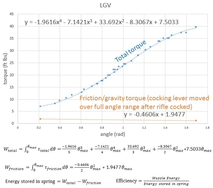
Fig. 1.13 Torque as a function of cocking lever angle as a Walther LGV is cocked. Integrating the curves allows one to determine the energy stored in the spring and the efficiency.
So now that we have some nice diagnostic tools to gain more insight into air rifles, let’s see what they can tell us about our Walther LGU, Walther LGV and FWB 124 test rifles in the next chapter!
 RSS Feed