Blog Archives

"Simple Field Target".- Maryland State Champ's 2021

5/30/2021

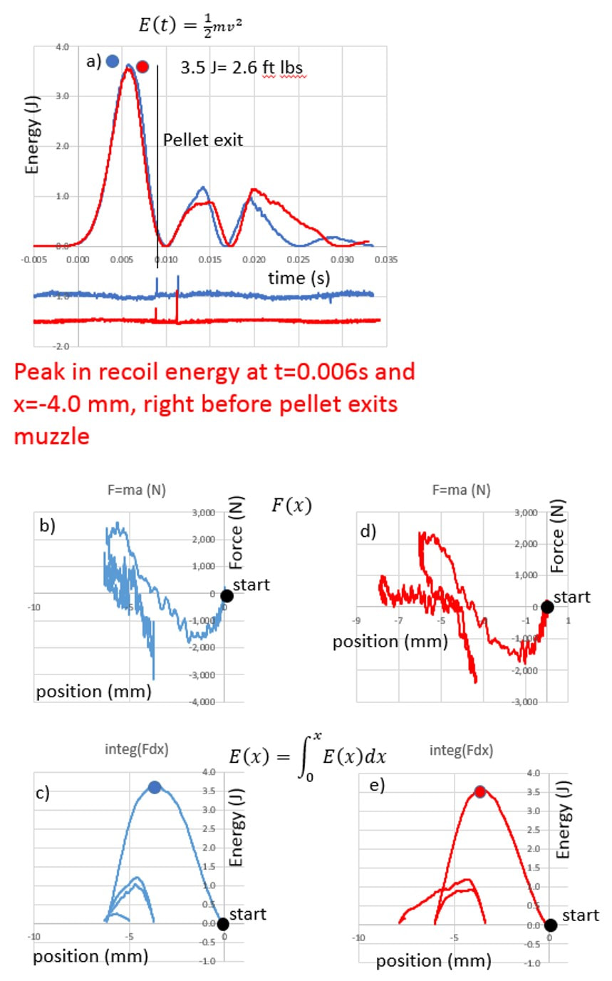
Shooting FT with a CCA/DIANA 430L

As I mentioned in an earlier post, I am liking this "Simple FT" thing!

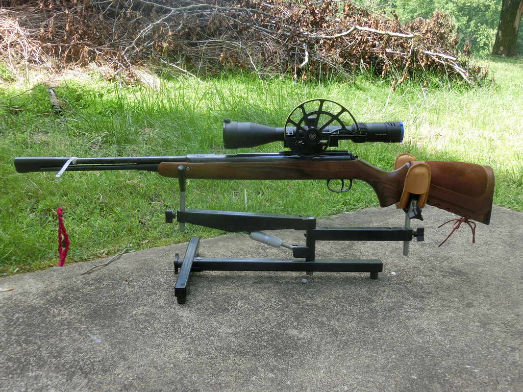
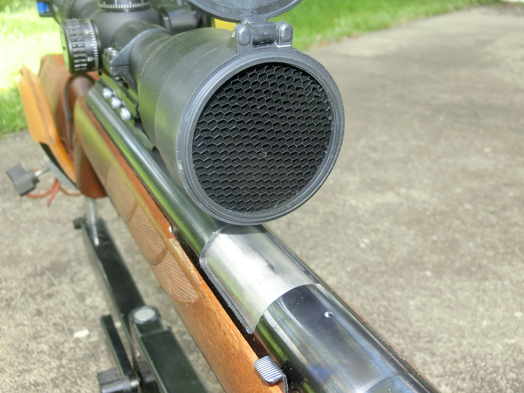
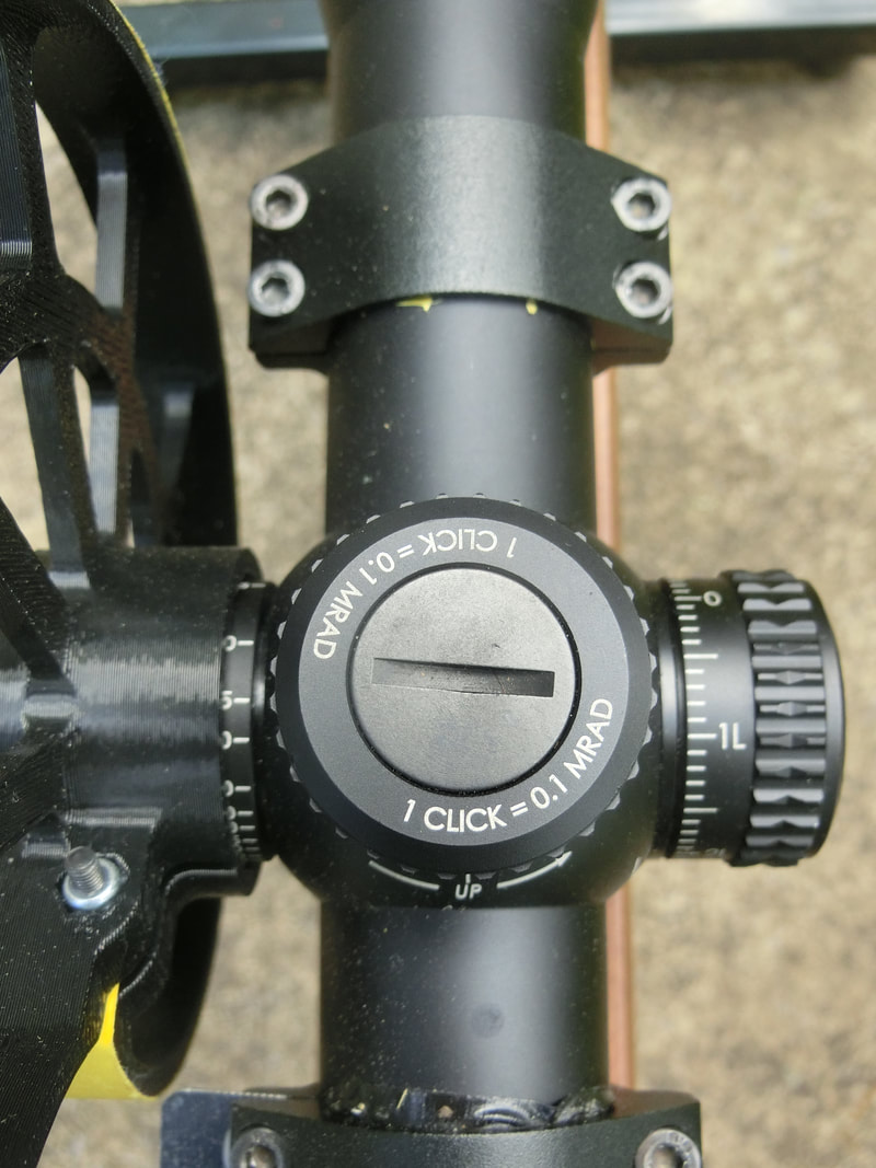
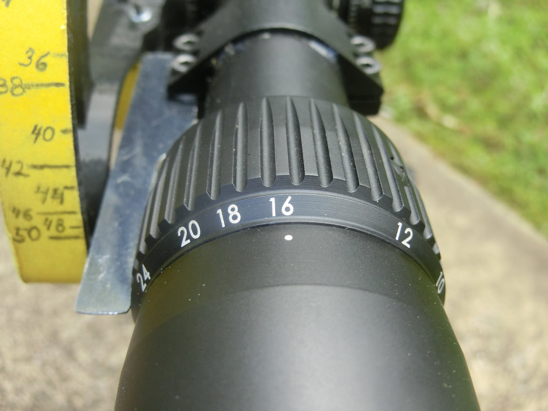
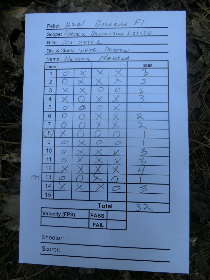
So, I decided to shoot the Maryland State Championship 2021 edition, with the same CCA/DIANA 430L, the excellent Vortex Optics Diamondback Tactical FFP 6-24 X 50 FFP EBR2C mrad and the very consistent H&N Baracuda FT (4.51/9.57) pellets.

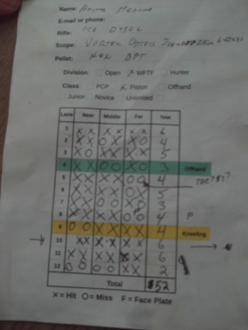
I THINK the system acquitted itself quite nicely, as can be seen from the Match Results:

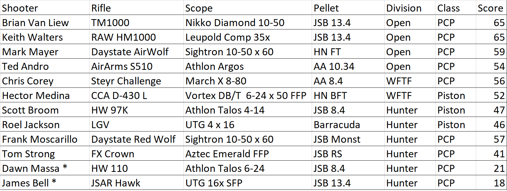
To put this in context:
Shooting from an industrial/floorer knee pad, with no straps, jacket, or special stock (no hook, hamster, nor heavy weight) and a 24X scope, no clicking; this gun's 52 points was highest among spring-piston shooters, and only 4 points behind the only other score in the WFTF Division.
And the power level did play an important role in this match, as several targets failed to fall with the sub 12 ft-lbs hits if the hit was lower into the KZ, or if it was at the farthest reaches.

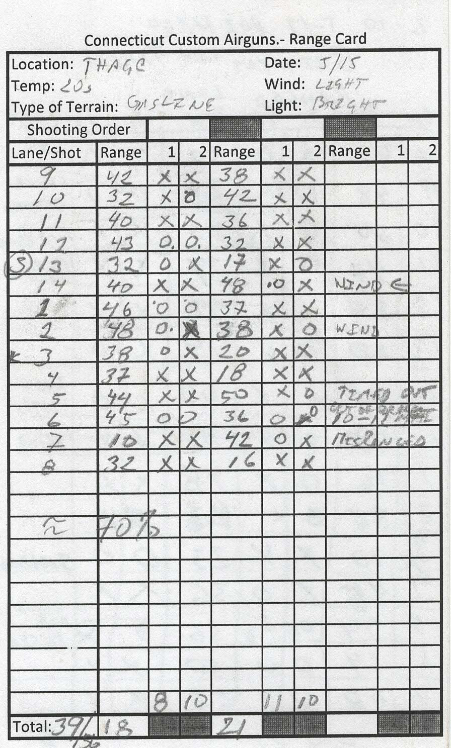
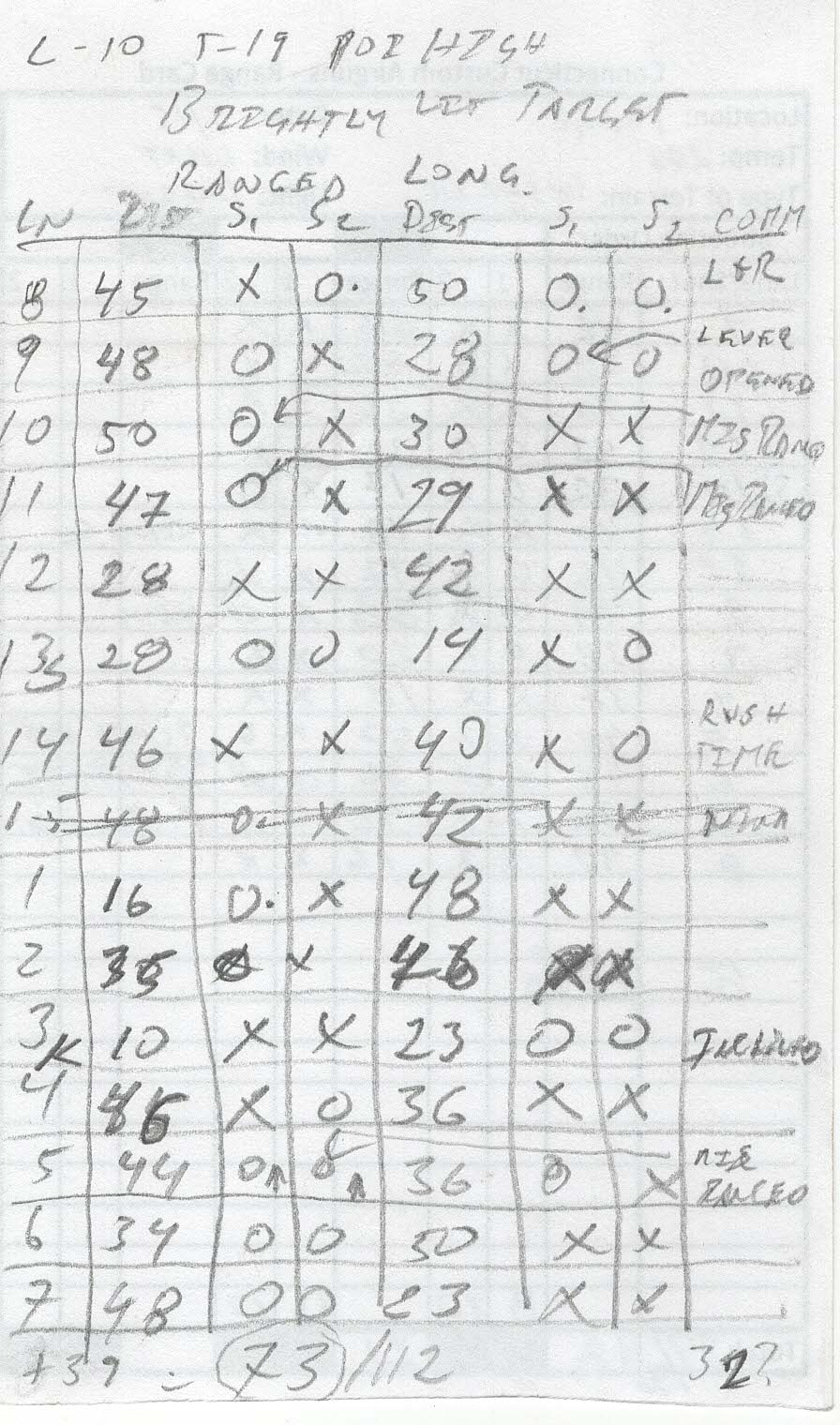
This is the second match I shoot with this system, so I am now more familiar with the trajectory and the wind drift.

Reading into my D.O.P.E.:

It is clear that the small KZ's at short range are not as high a challenge as the long shots.
With a humble piston sporter, the success rate at the near targets was 79%, while the success at the far targets was only 67%.
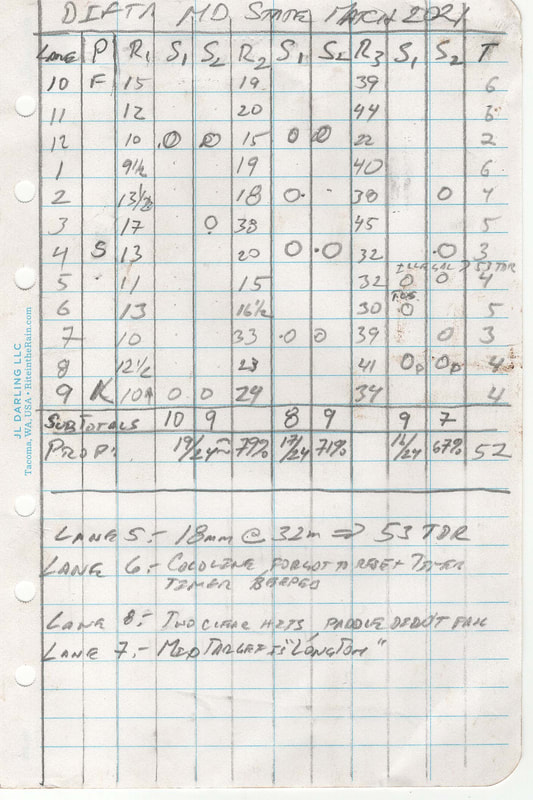
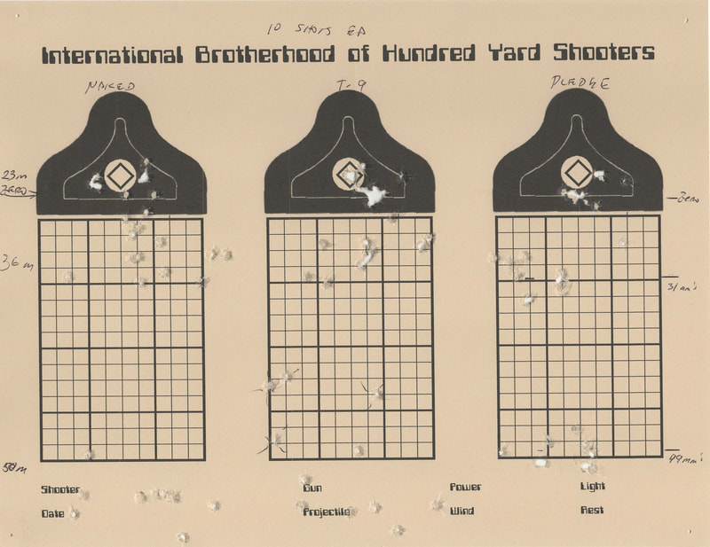
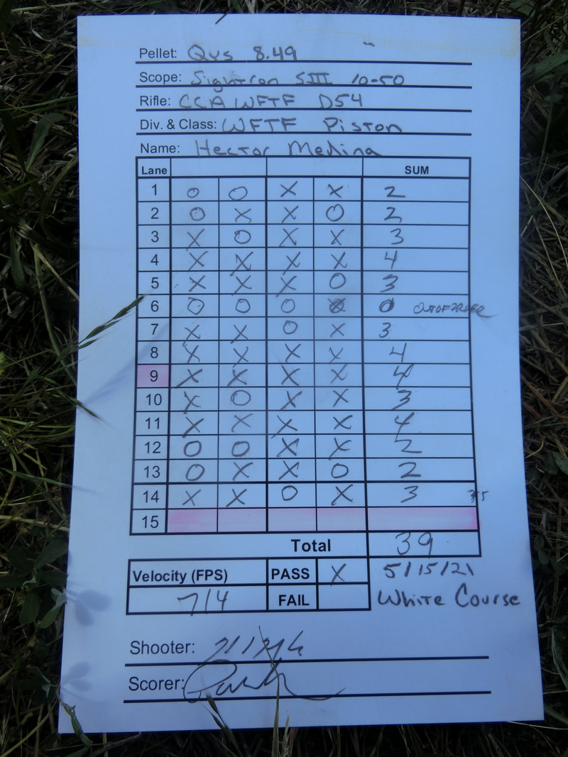
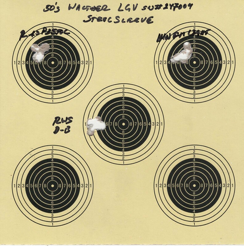
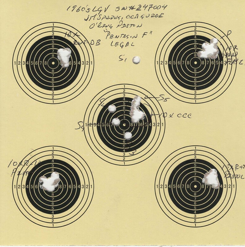
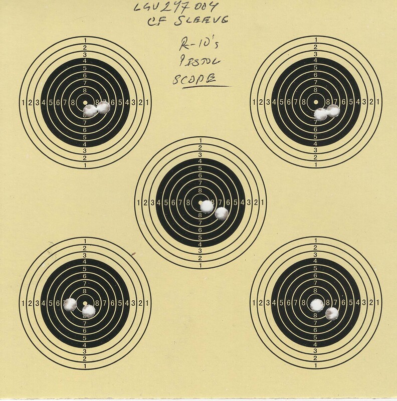
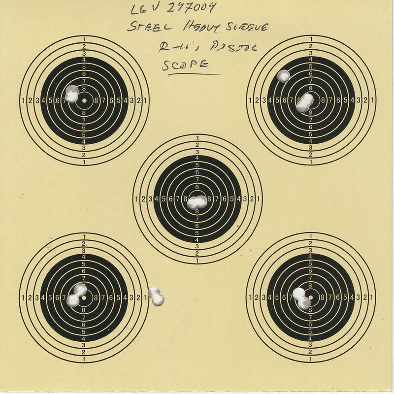
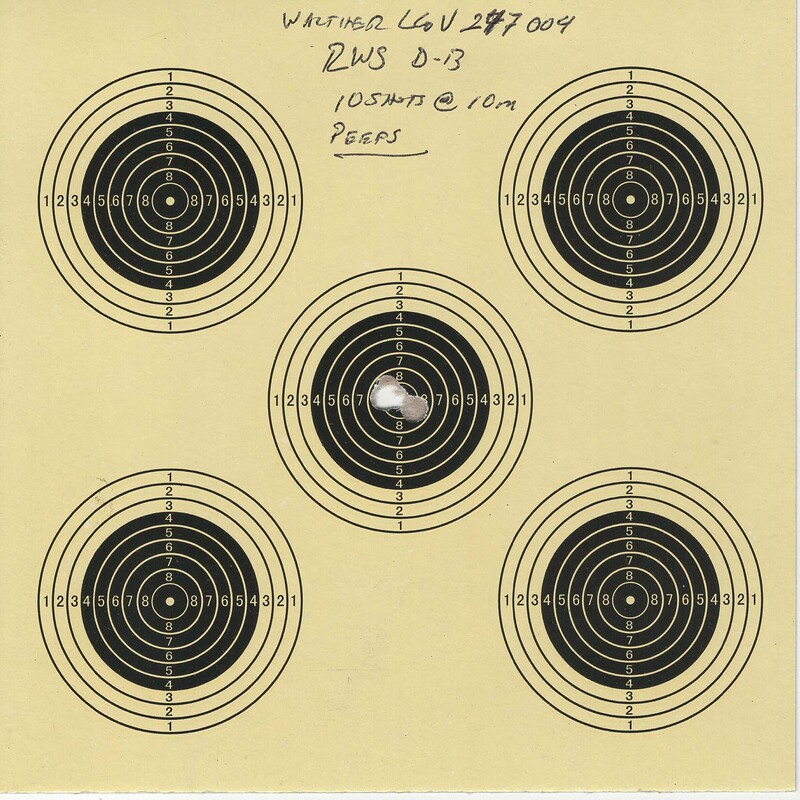
A small explanation of all the info that goes into the DOPE might be useful:
P=position (Free, Standing, or Kneeling); R=Range (in meters), S=score.
By not putting down the hits you mentally challenge yourself to keep the card "clean".
Paper is waterproof and you write with either a "Sharpie", or pencil, to keep the whole thing waterproof.
The little dots by the "zeroes" is the believed POI for that miss.
The small "P"s means that I protested the target.

Notes are important, and I try to put them down just after the shoot, so I don't forget things.
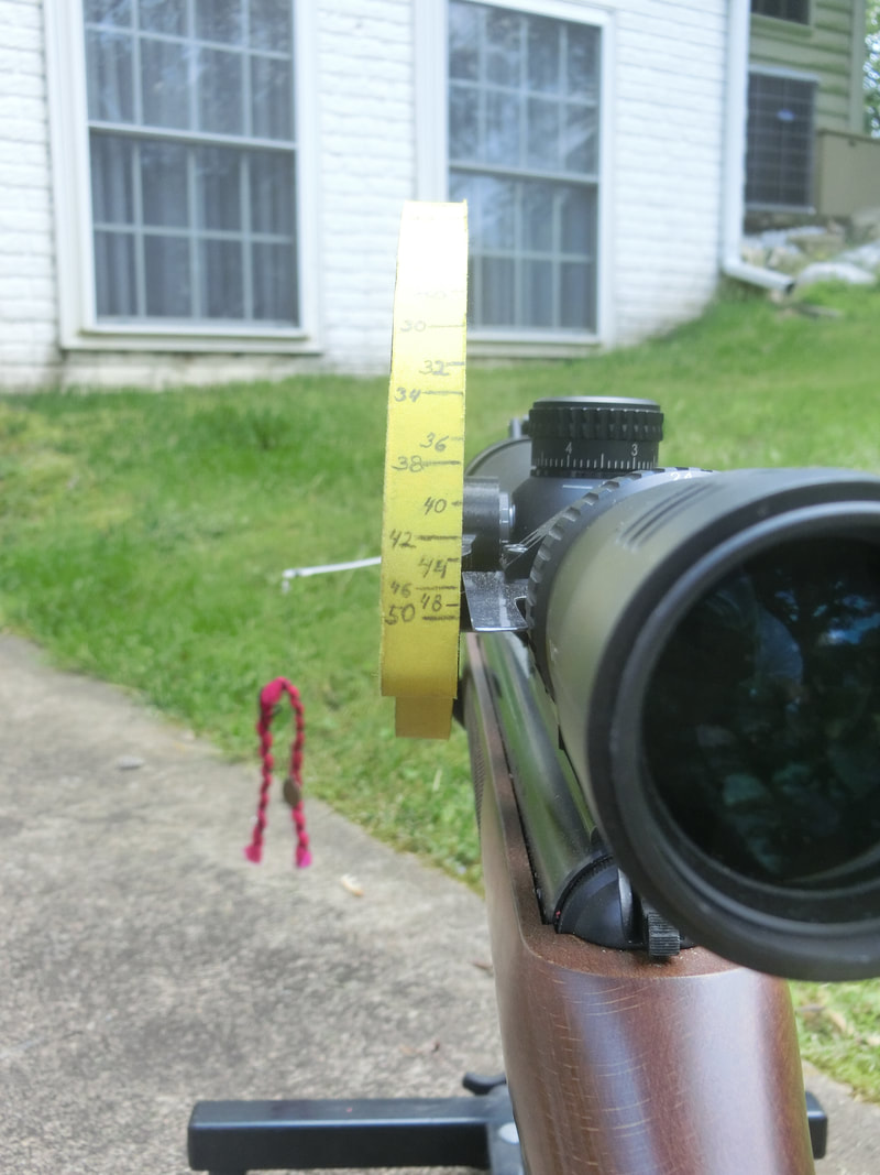
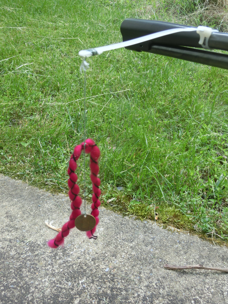
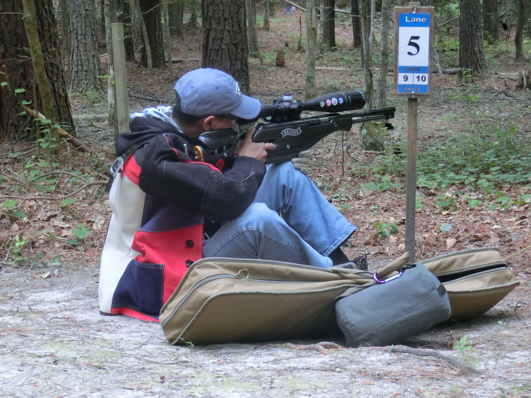
EG: The far target on lane 5 was suspected by Keith Walters (my shooting squad mate) to be illegal, when ranged and the KZ measured through the reticle, I thought it was about a 53 TDR (½ mrad @ 32 meters is about 5/8" at 35 yards), when the targets were brought in I measured the KZ at 18 mm's (my pocketknife has a mm's ruler LOL!) so, a bit less, but very close the max stated in page 6, "Targets", Section "I" of the new rules (Feb 2021).
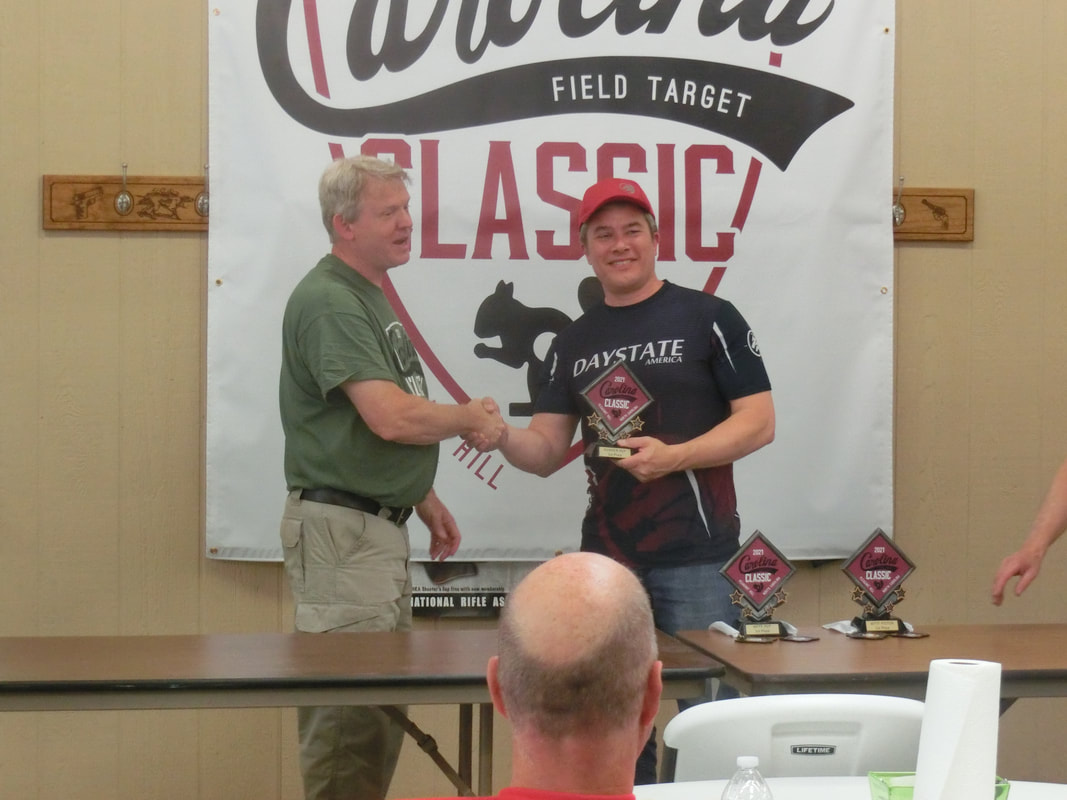
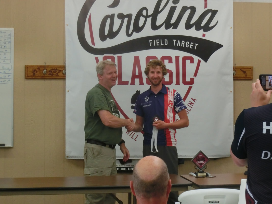
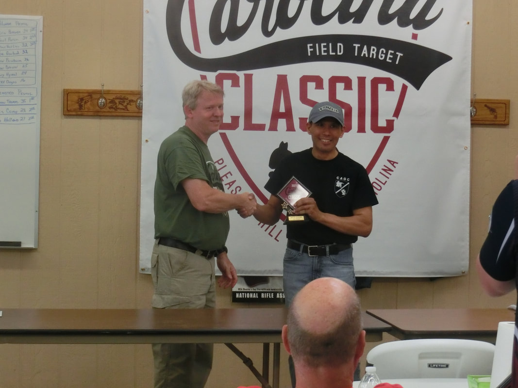
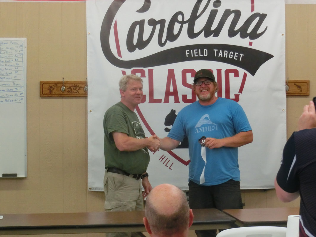
Keith brought it down, TWICE! He is a great shooter (together with Brian Van Lieuw, they posted the highest scores of the match; great shooting in anyone's book!), hopefully he will make the switch to WFTF after the end of the season, as the 2024 World's are slated to be held in the USA and it would be interesting to have him there.

So, the shoot was not an easy one, the scope was ranging accurately (within 1 meter either way), the rifle was putting the BFT's where it was aimed, and I was very happy with the performance of the system.

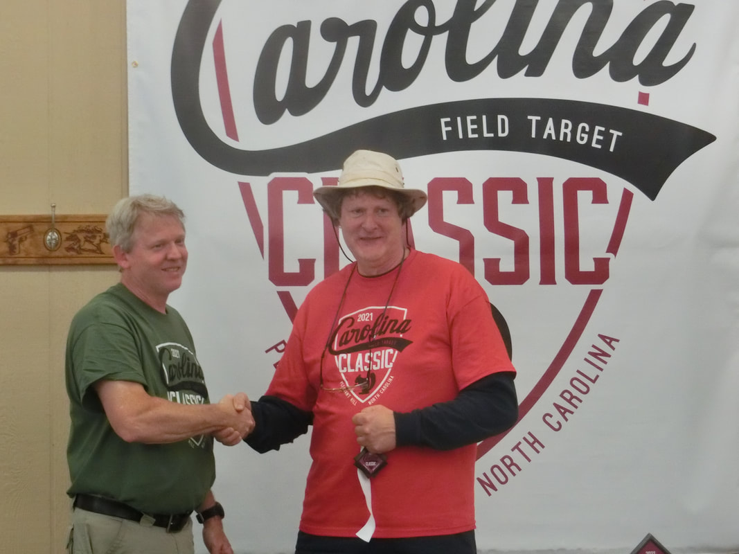
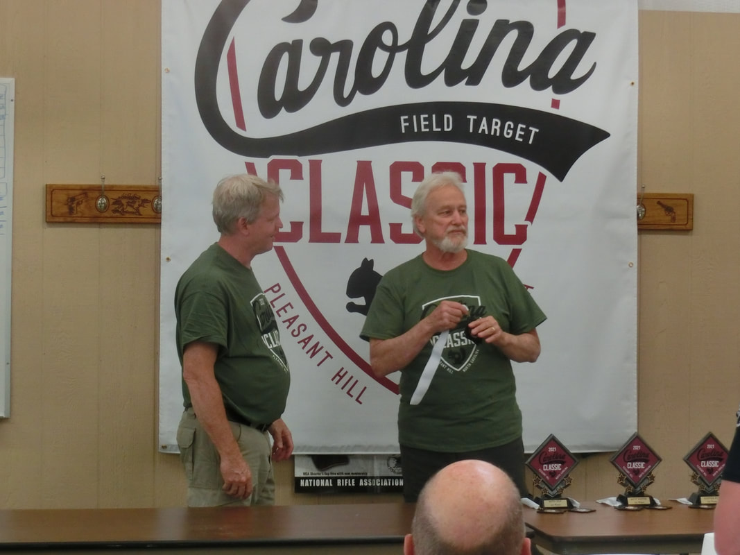
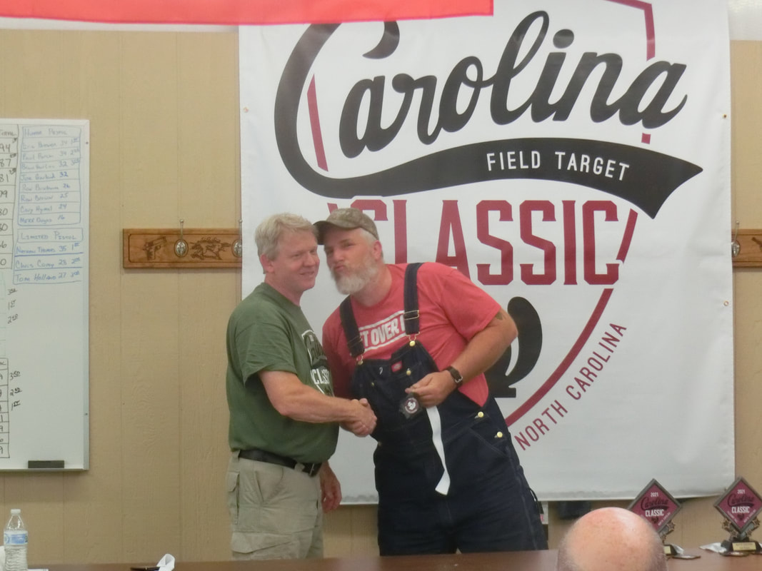
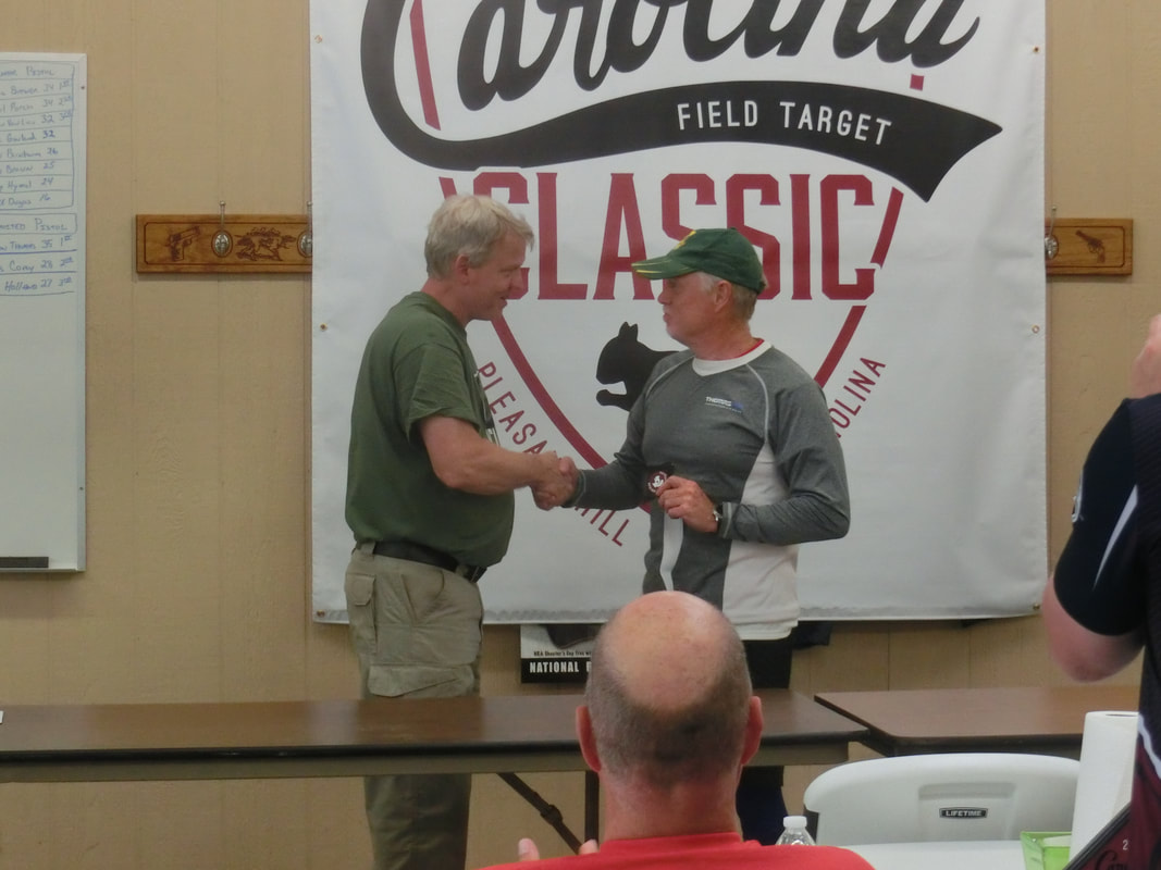
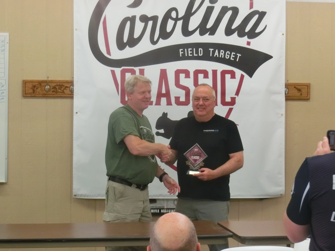
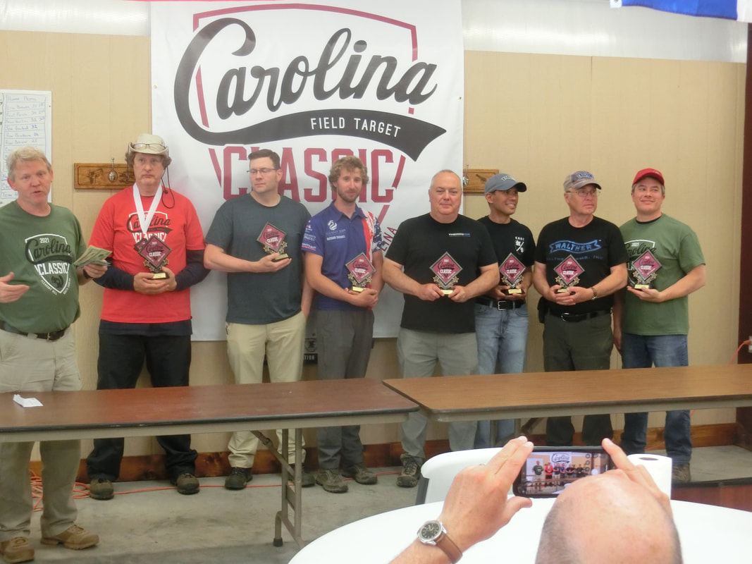
Now let's see some pictures:

Apoogies for the lack of focus, my 5 YO son had set the waterproof camera to "Macro" ROFL! But the picture does show the type of weather we encountered on arrival.

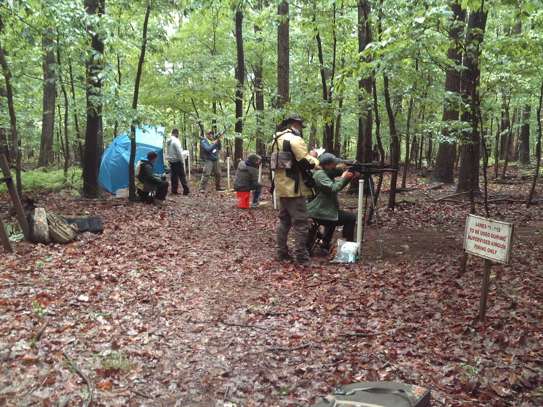
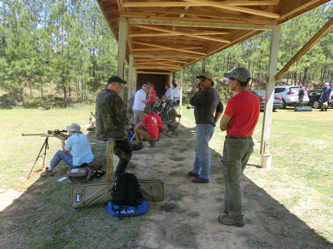
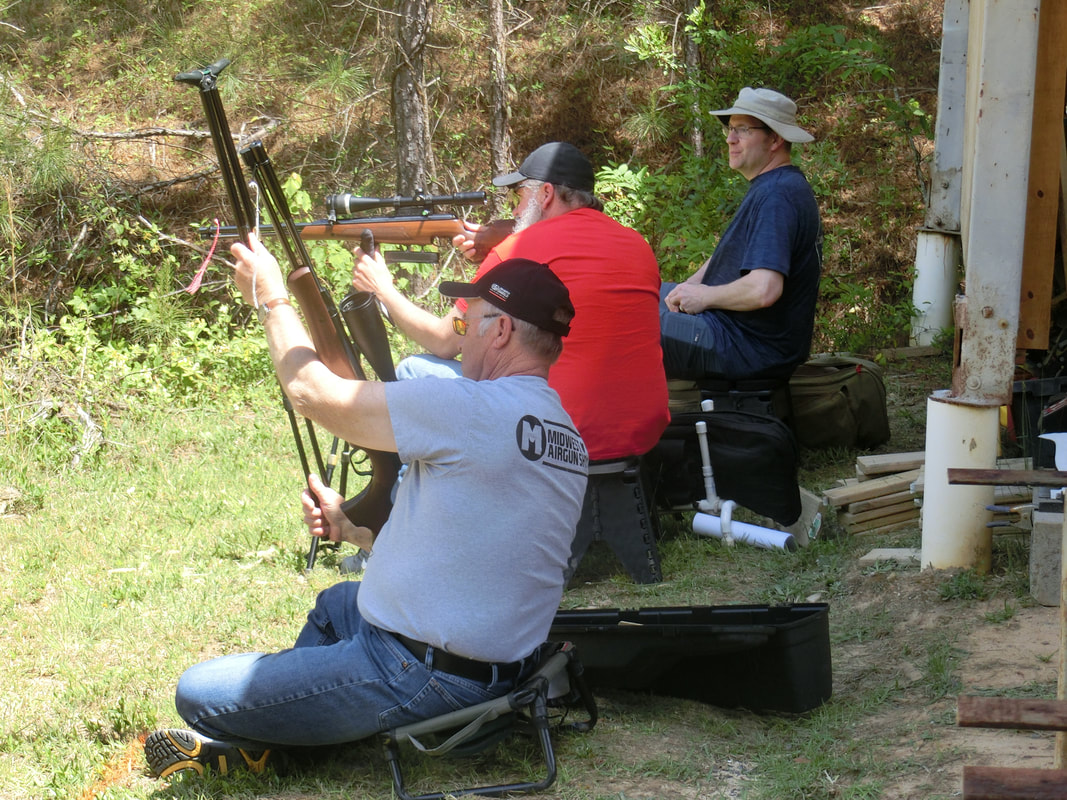
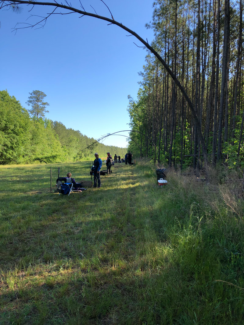
The shooting line was well populated. I need to get one of these umbrellas. Though I am not sure how one can take something like this to an International Match. LOL!

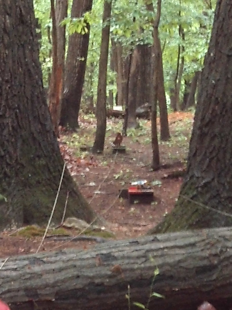
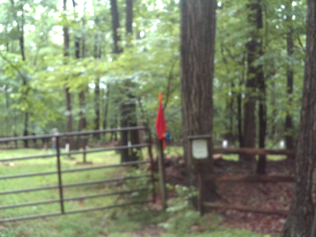
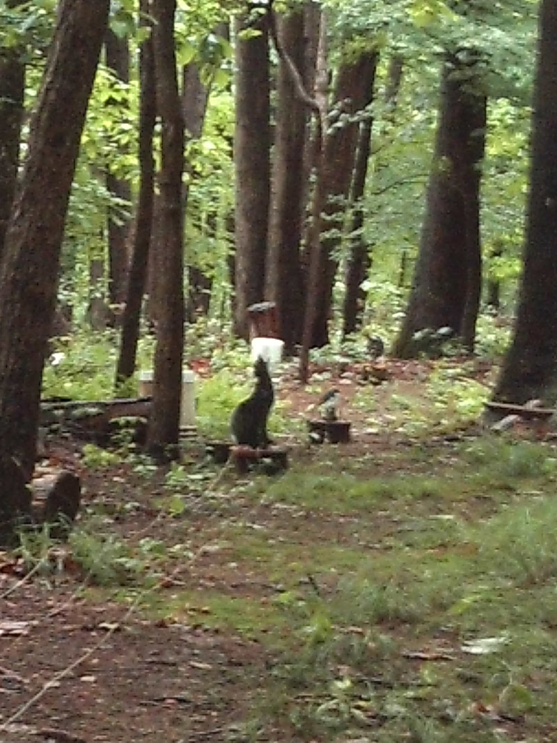
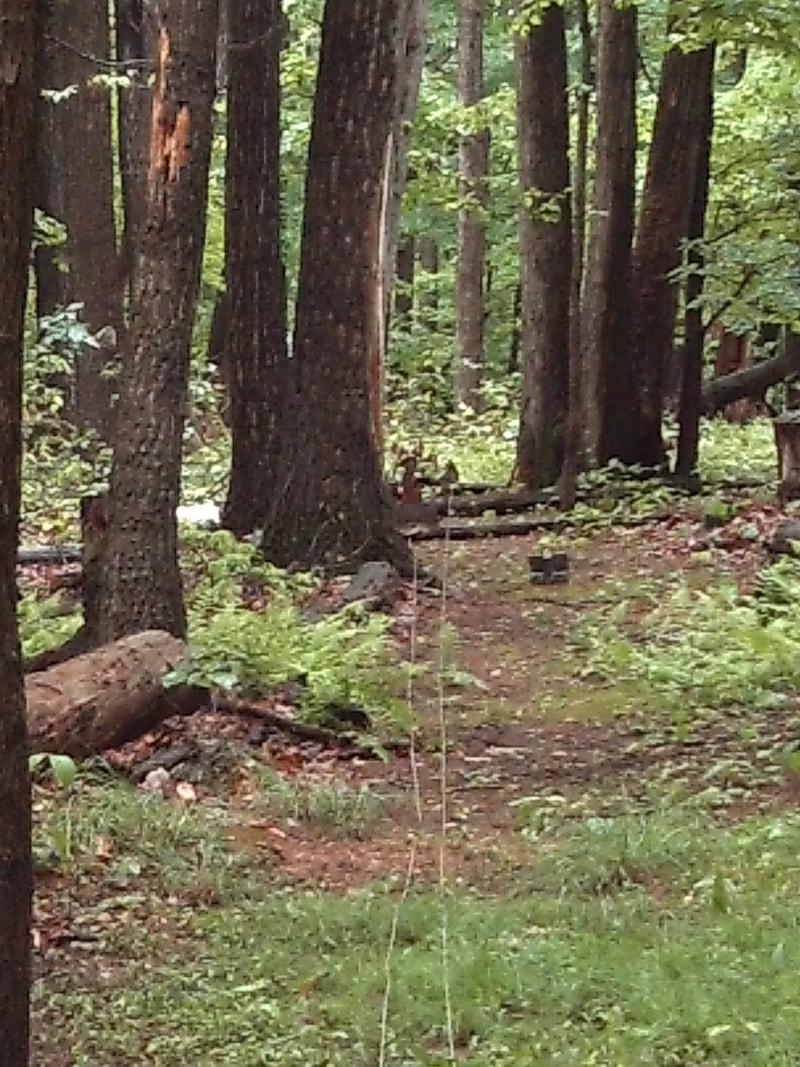
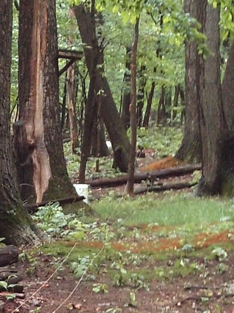
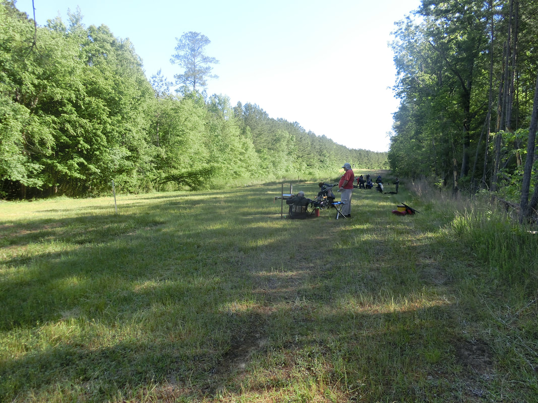
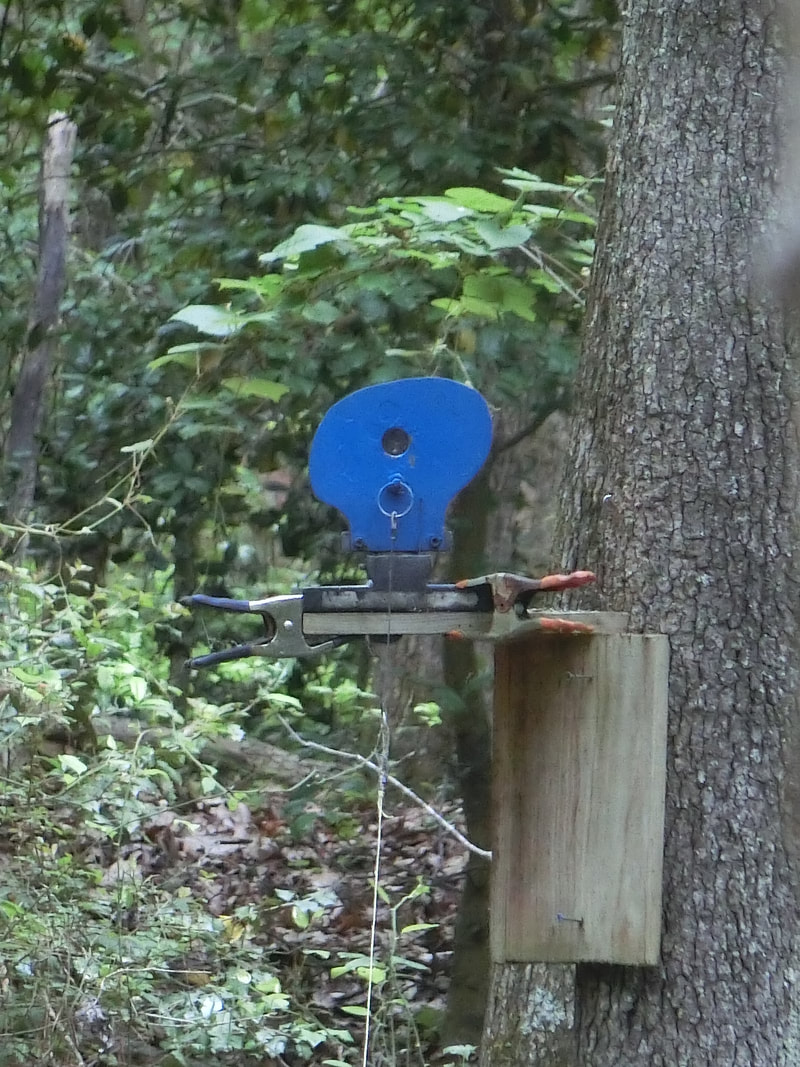
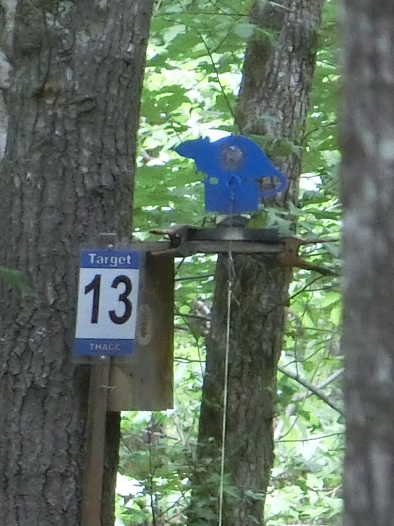
Zoomed in view of a typical lane. Apologies for the blurry picture, but the waterproof camera does not have a good zoom.

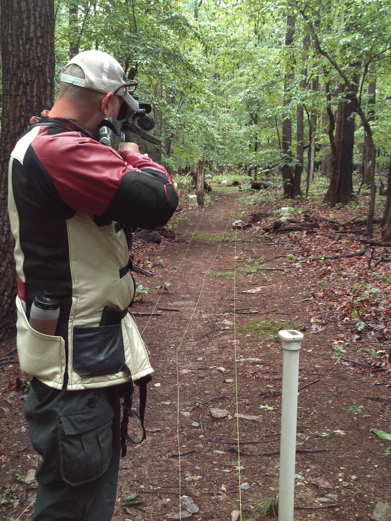
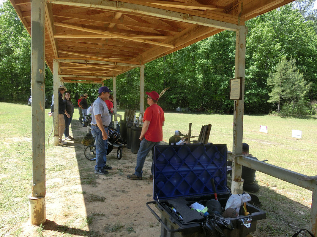
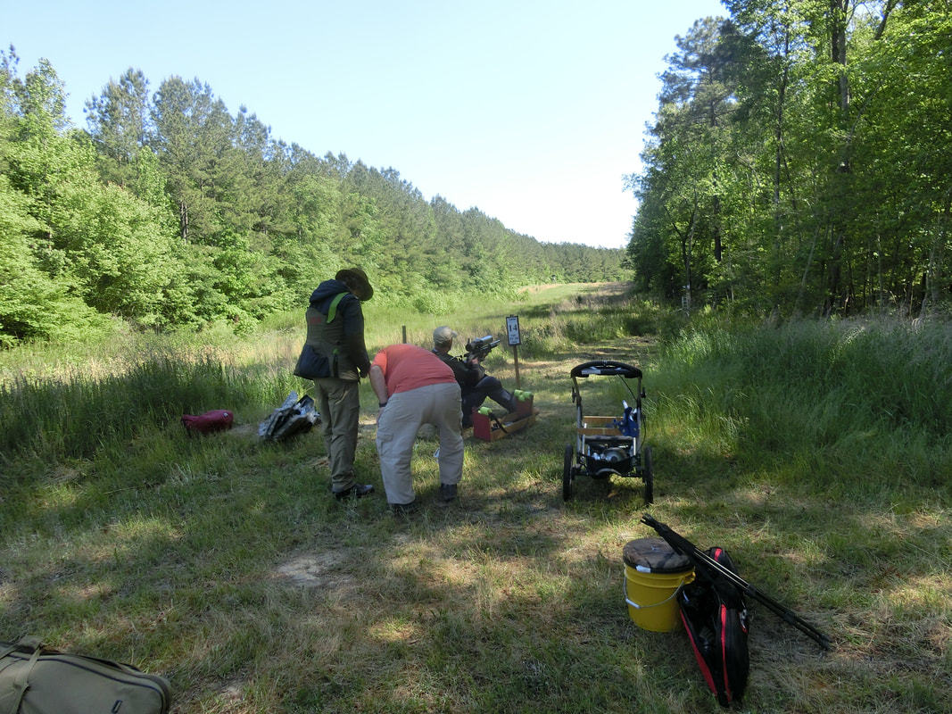
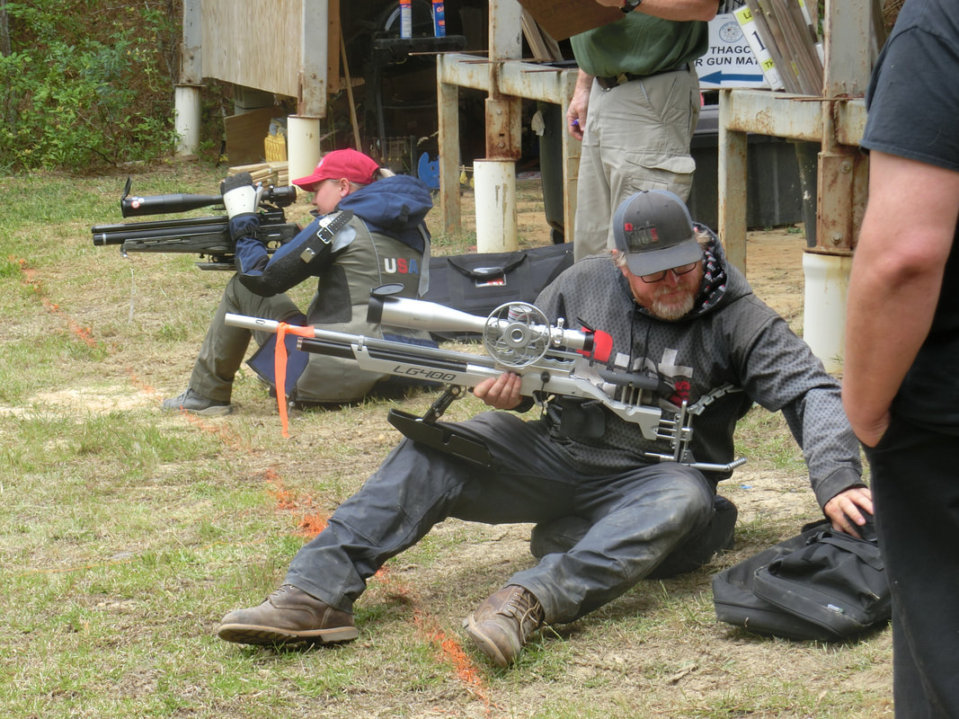
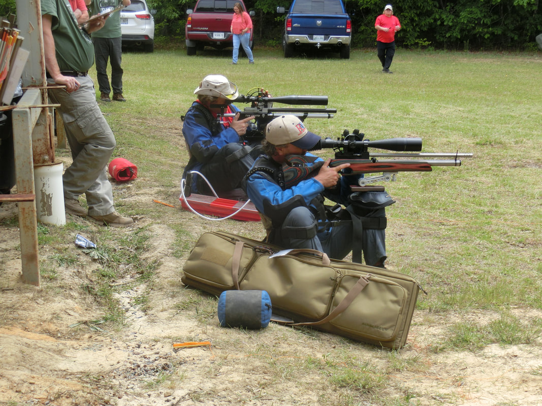
Keith's offhand position, a lot to learn from this picture.

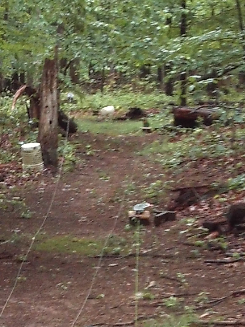
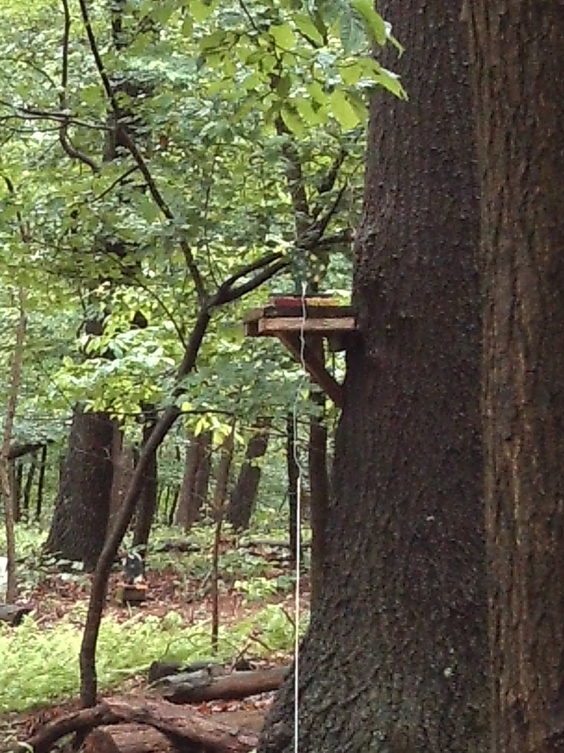
A zoomed in detail of the offhand lane arrangement.

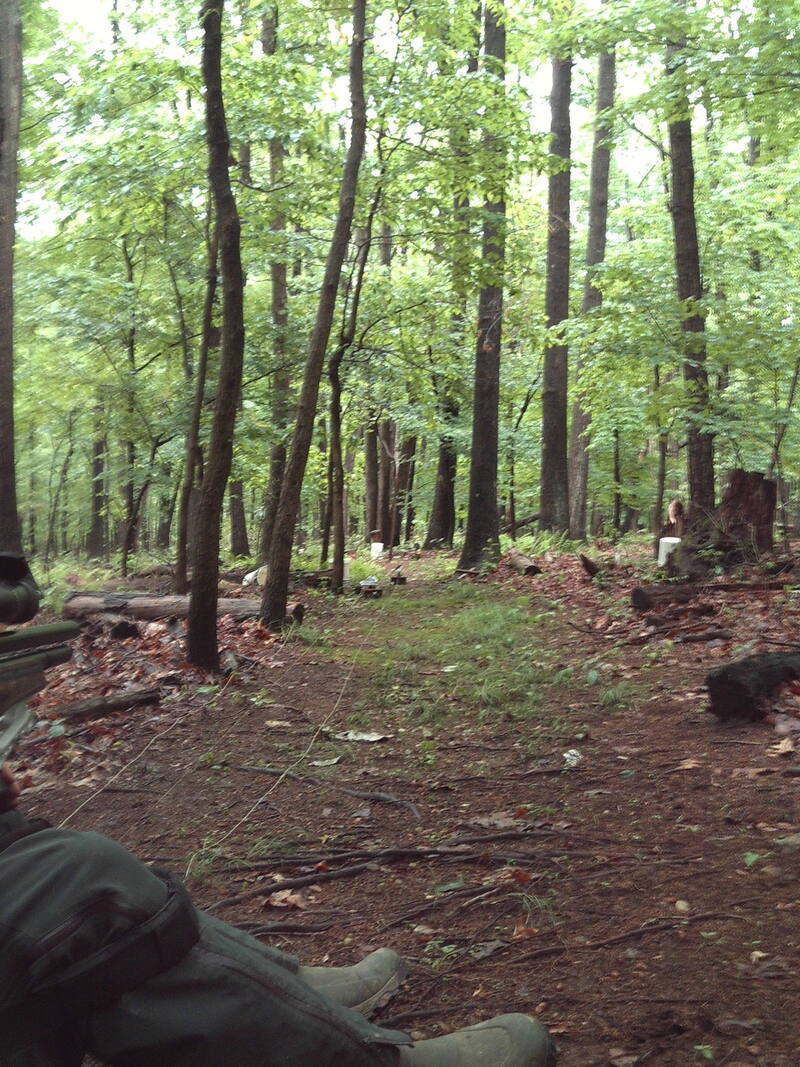
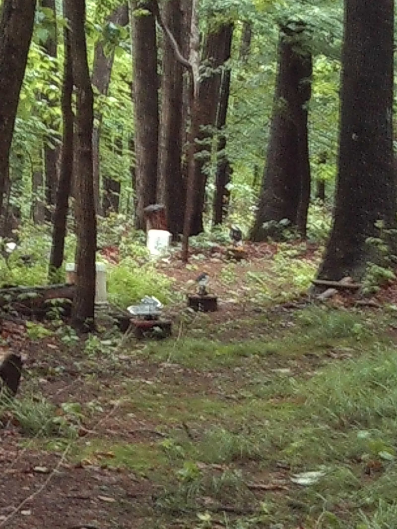
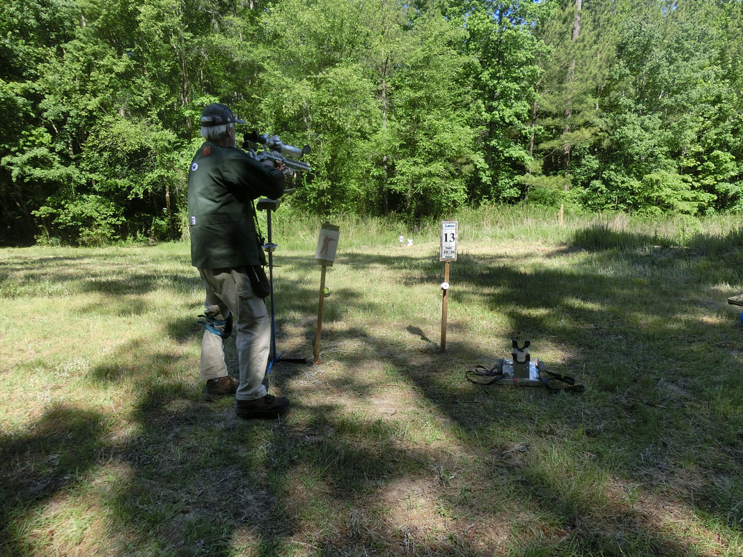
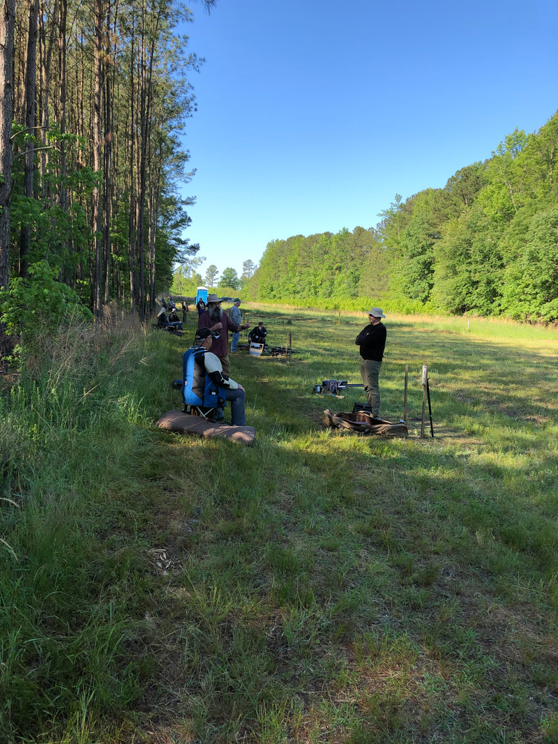
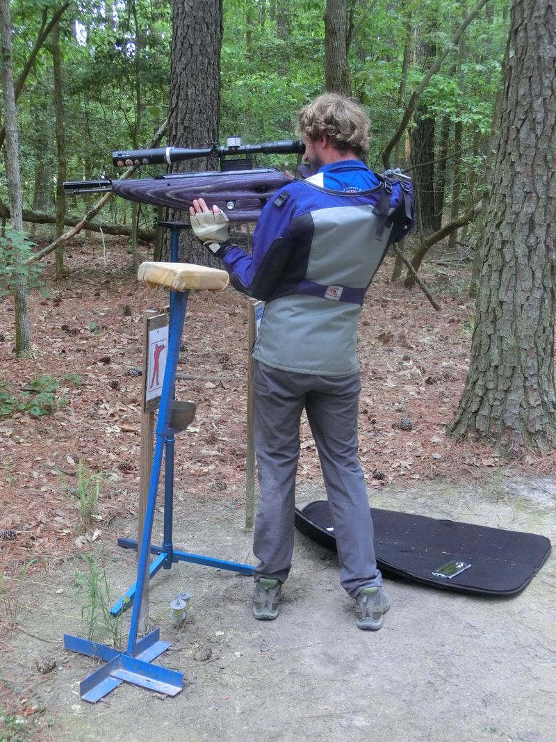
A typical "free position" lane.

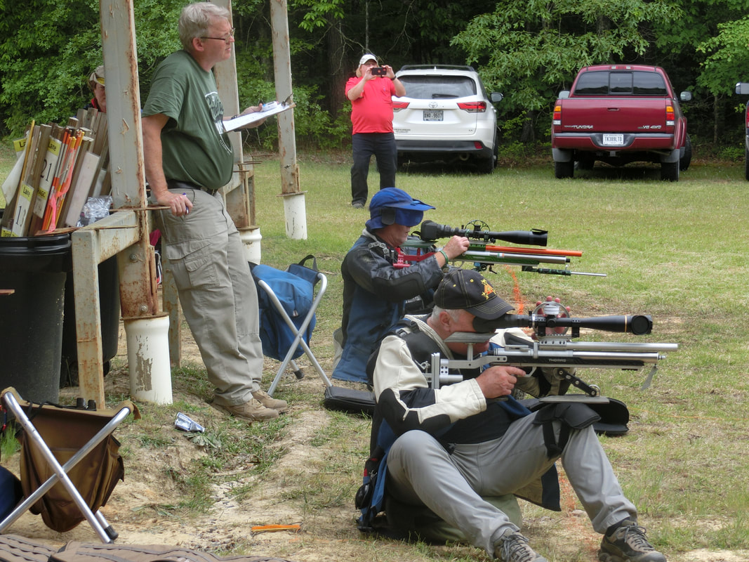
Some pictures of the lanes:

I know the system can shoot better, got most of my kneelers and half the standers; and I also realize that towards the end of the shoot (we started on lane 10), some fatigue was setting in, so further work into the cocking linkage has to be done to improve that.

It has also been an interesting "trip" to shoot the H&N BFT's; they are not for every barrel but, when you find a barrel that shoots them well, even at 730 fps, they can hold their own.

AND, this also shows that "simple" equipment can take you far in the FT game. That the FT game is not about power, but about accuracy, precision and Marksmanship.

So, next time you have the opportunity to go to a shoot, just "giddy-up-go" because you are sure to have fun, learn more than a few things, and meet some great people!

Keep well and shoot straight!

HM

2 Comments

Shot cycle Dynamics in 3 Spring-Piston Airguns Chap 4

5/27/2021

1 Comment

APOLOGY.-
The editor wishes to apologize to the readers for the delay in publishing this chapter.
The editor takes full responsibility for this delay, in no way was this the Author's fault.
So, let's get back to business:

LGU/LGV power plant swap: How does changing power plants affect performance and does a longer offset transfer port make a difference?

This adventure was initiated by Yogi's (of GTA fame) question about how transfer port (TP) geometry affects the performance of spring piston air rifles. Most break-barrel and some underlever (HW 77-97 series) air rifles have the TP located above the center of the compression tube, whereas the newer underlevers (TX200, LGU) have a TP that is centered on the compression tube. Jim Tyler has written several articles in Airgun World Magazine where he varied the TP diameter and length in the same rifle, but to our knowledge, no one has done a detailed comparison of central and non-central TPs. Hector realized that the Walther LGU and LGV were nearly identical except for the TP geometry, so he suggested we compare these two rifles more closely to try to answer Yogi’s question. In this chapter, I swapped the piston, mainspring, and trigger group between the LGU and LGV. In principle, using the LGU power plant in the LGV, and vice versa, should help isolate the effects of the TP geometry. Ideally, everything except the TP geometry should remain the same when the swap is made. So if one takes the power plant from the LGU and puts it in the LGV, the main difference will be that the LGU spring is pushing air through a longer, offset TP compared to when it was in the original LGU compression tube. The same is true when the LGV power plant is placed inside the LGU. Does the LGV power plant do better when it’s pushing air through the short, centered TP in the LGU? Unfortunately, other things also change when the swap is made. For example, the fit of the piston seal in the compression tube is slightly different. Ideally one would take the same rifle and move the TP around, as Mr. Tyler did with TP length and diameter, but this would be very difficult and would involve building a highly specialized rifle.

Figure 1 looks at the accuracy of the LGU before and after swapping its power plant with the LGV. Accuracy is better and velocity is about 20 fps lower before the swap. The standard deviation in muzzle velocity is nearly identical, suggesting that the consistency of the power plant does not depend on which rifle uses that power plant.

Fig. 4.1 LGU accuracy based on 10-shot groups from the bench at 20 yards before a) and after b) the swap with LGV piston, spring and trigger group.

Figure 2 shows the accuracy of the LGV before and after swapping its power plant with the LGU. The LGU gained about 20 fps with the LGV power plant but the LGV dropped by more than 66 fps with the same batch of QYS Dome pellets when it used the LGU power plant! This suggests that the LGV was better tuned for its power plant and is more sensitive to power plant changes than the LGU. Overall, accuracy was better before the swap, but the first three groups with JSB Exact 4.53 mm after the swap sure look good!

Fig. 4.2 LGV accuracy based on 10-shot groups from the bench at 20 yards before a) and after b) the swap with LGU piston, spring and trigger group.

Now let’s take a look at the efficiencies of the two rifles before and after the swap, as shown in Fig. 3. The efficiency of the LGU dropped dramatically with the LGV power plant. Cocking work increased by about 22% but the muzzle energy increased only by about 5%. The efficiency of the LGV also dropped when using the LGU power plant, but not by as much. Even with the LGU power plant, the efficiency of the LGV was still pretty good, especially with the JSB pellets. It’s interesting that the most efficient pellet depends on the power plant. I would have naively expected that it just depends on the pellet friction in the bore, but it’s clear that with its original power plant, the LGV was slightly more efficient with QYS Dome pellets, but with the LGU power plant, the LGV was significantly more efficient with JSB 4.53mm pellets. The LGU’s greater efficiency loss in using a borrowed power plant could be due to the TP, but there may be other reasons. For example, this could also happen if the LGU piston seal is a bit undersized compared to the LGV piston seal. In that case, the LGU piston seal would slide with very low friction in the LGV compression chamber whereas the larger LGV piston seal would be a tighter fit in the LGU compression chamber, which would then encounter more friction and produce lower muzzle velocities. I didn’t notice much of a difference in piston seal friction when inserting the pistons, but if I were to do this experiment again, I would have kept the piston seals on the original rifles, that is, put the LGV piston seal on the LGU piston when inserting the LGU piston into the LGV and put the LGU piston seal on the LGV piston when inserting the LGV piston into the LGU.

Fig. 4.3 Cocking work and efficiency of LGU and LGV with original and swapped internal parts.

Another possibly important factor in the swap is that the LGV uses an anti-bounce piston (ABP), which we expect to increase muzzle energy by about 10% (see Chapter 2). Maybe the ABP is working better in its original home, the LGV, than in its new host, the LGU? To get a better idea of how the rifles are recoiling, which also could give some clues about how the ABP is working, I measured the recoil traces of both rifles before and after the power plant swap, as shown in Fig. 4. The recoil of the LGU gets significantly stronger with the more powerful LGV spring, as can be seen by the position, velocity and acceleration plots in Fig. 4a). The second dip in the acceleration is clearly deeper with the LGV spring. On the other hand, the first positive peak in the acceleration is a little bit smaller with the LGV spring. Maybe the ABP is moderating the abrupt slowdown of the piston before it starts heading backward? These strong changes in recoil result in a small increase in the muzzle velocity. Unlike the LGU, the LGV shows very small changes in recoil (Fig. 4b) that are accompanied by a much larger decrease in muzzle velocity. There is hardly any difference between the original and swapped power plants in the first few oscillations of the LGV’s acceleration despite the fact that the muzzle velocity drops by 66 fps when the power plant is swapped.

Fig. 4.4 Recoil traces showing the position, velocity, and acceleration of the sled-mounted rifles over 250 ms for the a) LGU (AADF) and b) LGV (JSB Exact) with original (blue traces) and swapped (red traces) piston, mainspring, and trigger group.

Figure 5 zooms in on the early parts of the recoil traces for the LGU (Fig. 5a) and the LGV (Fig. 5b). Also shown in the velocity vs time plots are the light gate traces, which show when the pellet exits the muzzle. The timescale for the recoil plots was shifted to align the pellet exit times for the original and swapped components. It’s surprising how little the recoil changes when power plants are swapped, suggesting that the dominant factor in recoil is not the power plant, but the rest of the rifle!? It looks to me like the LGU recoil remains distinct from the LGV recoil regardless of which power plant it uses. This is especially puzzling since the LGV power plant uses an ABP and the LGU power plant doesn’t. For example, the shoulder just before the first peak in the LGU velocity (see black arrow in Fig. 5a) occurs with both power plants. Also, the distinctive flattening at the top of the first velocity peak for the LGV (see black arrow in Fig. 5b) occurs with both power plants. The LGU power plant does appear to enhance this flattening, so maybe this is where the ABP makes a difference? Furthermore, the LGU spring is nearly dry with a very light coating of Superlube whereas the LGV mainspring has a heavy coating of tar. This doesn’t show up very strongly in the recoil traces. Part of this apparent insensitivity in recoil to the power plant is due to the far greater total weight of the LGU rifle, which simply rescales the vertical axes in the recoil plots; it’s harder to get a heavier rifle moving. The LGU will always be heavier than the LGV, regardless of power plant! However, the qualitative shape of the recoil traces seems to not depend much on the power plant and this is perhaps where we’re seeing the TP geometry making its biggest impact? Of course, all this analysis has to be taken with a grain of salt since the rifle is moving forward in the sled given the huge forces pulling on the Velcro strap at the piston bounce, as Steve in NC pointed out in the Airgun Warriors thread.

Fig. 4.5 Recoil traces showing the position, velocity, and acceleration of the sled-mounted rifle over 50 ms for the a) LGU (AADF) and b) LGV (JSB Exact) with original (blue traces) and swapped (red traces) piston, mainspring, and trigger group. Pellet exit times are marked by vertical black lines. Black arrows show distinctive features in the velocity traces.

In the final two figures we look at the recoil energy for the LGU (Fig 4.6) and LGV (Fig. 4.7). Since we know how the entire rifle moves during recoil, we can determine its kinetic energy as a function of time or position. This is important and interesting since the movement of the rifle can affect the POI. There are three ways to determine recoil kinetic energy of the moving rifle and sled. The easiest way is to use the formula E=½ mv^2, where E is the kinetic energy (the energy of motion), m is the mass of the rifle and sled added (since they’re moving together) and v is the velocity of the rifle and sled. Figure 4.6a) shows the kinetic energy of the rifle and sled system as a function of time. Note that this energy is always positive; whenever you square a real (positive or negative) number like velocity you get a positive answer. The kinetic energy oscillates just like the velocity. As the rifle recoils backward, the peak energy absorbed by the rifle occurs at around 0.007 s, which corresponds to a sled position of -3.6mm according position vs time plot at the top of Fig. 4.5a). This peak energy is 2.4 J (1.8 ft lbs) for the original innards and 3.0 J (2.2 ft lbs) for the swapped LGV innards. I placed red and blue dots to mark these positions. The second way to determine the recoil energy is to use the instantaneous power at time t, P(t), which is just the product of the force and velocity at that time. One can then just integrate the power from the starting time to time t to get the energy expended in recoil during that time window. Although I don’t plot the result, it looks exactly like the plot in Fig. 4.6a). The third way to get the recoil energy is to plot the force F as a function of position x, F(x), and then integrate that force from the starting position to some position x to get the energy expended to get to x. The integral along x is bit trickier since the dx intervals vary (remember that we record with a constant time interval between points, but the distance between the positions of neighboring points will vary as v varies). I used this method to determine recoil energy vs position by plotting the force as a function of position x (not time!), as shown in Fig. 4.6 b) and d) integrating the force over position, as shown in Fig. 4.6 c) and e). In Fig. 4.6 b) and d), the plot retraces itself as the rifle moves back and forth in position. Using this technique we see that the peak recoil energy occurs when the sled position around -3.6 mm, as can be seen in Fig. 4.6 c) and e). I placed red and blue dots to mark these positions. I'm very relieved to see that the positions and times of these peaks, as well as the peak values agree pretty well using the three methods. Newton was right! The further oscillations in energy appear to be pretty consistent when comparing E(t) and E(x). The recoil energy peaks about 0.003s before the pellet leaves the barrel. So this peak recoil energy could have a big impact on accuracy, as the rifle reaches its maximum kinetic energy right before the pellet leaves the barrel. The more the rifle moves before the pellet leaves the barrel, the harder it will be to stack pellets on top of each other! In Fig. 4.6 one can see that the peak recoil energy increases by about 25% when the LGV spring is used in the LGU. Unfortunately, this strong (25%) increase in peak recoil energy is accompanied by a very weak (5%) increase in muzzle energy.

Fig. 4.6 Recoil energy of LGU with original (blue) and swapped (red) internals: a) recoil energy vs time and pellet exit traces, b) and d) force vs position, and c) and e) recoil energy vs position. The peak recoil energies are indicated red and blue solid circles and are the same whether one uses kinetic energy in a) or integrates force in c) and e).

In Figure 4.7 I do the same recoil energy analysis for the LGV with its original and LGU innards. In this case, “original” means the ABP piston, which certainly is not a standard piston in the LGV, but it’s what the LGV had when I got it. Again, the three techniques for obtaining recoil energy produce the same results. The time (Fig. 4.7a) and position (Fig. 4.7 c and e) of the recoil energy peak are 0.006s and -4.0 mm, respectively. These are very similar to the values obtained for the LGU and are consistent with the position of the sled at that time (Fig. 4.5b). In this case however, the original and swapped innards produced almost exactly the same peak recoil energy of around 3.5 J (2.6 ft lbs). This is surprising since the original ABP in the LGV produces about 19% more muzzle energy compared to the LGU piston and spring in the LGV. So for the same peak recoil energy, the ABP in the LGV produces about 19% more muzzle energy. Unfortunately, the ABP doesn’t produce a similar enhancement in the LGU, but this isn’t surprising since the ABP needs to be specially tuned for each rifle. The peak recoil energy is higher in the LGV (2.6 ft-lbs) compared to the LGU (2.2 and 1.8 ft-lbs), which is due to the lighter mass of the LGV. There’s another very interesting and possibly important difference between the LGU and LGV recoil energy traces. In the LGV, the pellet exits a bit later and the recoil energy peak occurs a bit earlier, so at the time of the pellet exit the LGV is moving less than the LGU. If the pellet were to leave another millisecond or so later, the LGV would actually be at rest at the moment that the pellet leaves the barrel. Unfortunately, all the motion before the pellet leaves the barrel could disrupt the aim, so there may not be much of an advantage in having the rifle stationary at the moment the pellet leaves the barrel. You really would want the rifle to not move at all from the trigger pull to the pellet exit, not just during the pellet exit.

Fig. 4.7 Recoil energy of LGV with original (blue) and swapped (red) internals: a) recoil energy vs time and pellet exit traces, b) and d) force vs position, and c) and e) recoil energy vs position. The peak recoil energies are indicated red and blue solid circles and are the same whether one uses kinetic energy in a) or integrates force in c) and e).

The main conclusion of this first swap test is that it may be too soon to make any strong conclusions. It is clear that the LGV is just as efficient as the LGU, so any arguments about the inefficiency of long, non-central TPs doesn’t apply here. There also was a strong asymmetry in the muzzle energy gain and loss when power plants were switched. The LGU gained much less than the LGV lost when the power plants were switched. Maybe the ABP was optimized for the LGV and didn’t produce the same degree of improvement in the LGU? It also is clear that the distinctive recoil traces of the two rifles was maintained even after the power plants were switched, which suggests that the rifle itself (maybe the TP geometry) is more important than the actual power plant in determining how the rifle recoils. It’s also interesting that the peak recoil energy significantly increased in the LGU when using the more powerful LGV spring and ABP, but that the increase in muzzle energy was very weak.
On the other hand, the ABP in the LGV produced the nearly the same peak recoil energy as the LGU piston and spring, but with a much higher muzzle velocity.

1 Comment

"Simple Field Target".- The North Carolina Classic 2021

5/17/2021

12 Comments

In a casual conversation with a good friend, an old "survivalist" from Texas, he questioned me (as old people are capable of), with the force of experience and the lapidary tone of a parent:
"Your FT sport, you've been at it for,. . . what?, something like two decades?"
I had to admit that, yes, a bit under 21 years. And he countered:
"And in those 21 years, has the sport advanced?
Hmmmmm, yes, I said, I assume it has advanced in some aspects and has retrograded in some others.
"OK" he said. "Let's concentrate on those aspects on which you think it has retrograded. What has become less interesting?"
In here I have to clarify that he refers to many things, and persons, as being "interesting" or "uninteresting", and that in that seemingly simple concept, he engulfs all sorts of aspects and feelings from 'fun and exciting', to 'loveable and cherishable'.
So, I told him: "It has become MUCH more complicated. The 'Simple' in it is gone"
As a good surgeon he once was, he began dissecting the issue:
"Is the 'simple' in IT or in YOU gone?"

And THAT made me think.

Yes, the courses have become harder, longer, more challenging, but the pellets and the rifles have advanced so, ¿Why do WE make it complicated? Is it truly that important to place "Top X" that we allow it to detract from the enjoyment of the sport?
¿Why do we want to solve all issues with equipment and more equipment?
¿Why not return to "Simple FT"?

I had been working by times and lapses, on how to improve the DIANA 430L, and my last conclusion was that it was still not an FT rifle. My objections were, mostly, what I had told my friend "detracted" from the sport!
AND that statement applied to a rifle scoped with a 2-7 X 28 scope.

So, I pulled the Vortex Optics Diamondback Tactical 6-24X50 FFP - Mil/Mil (probably the best spring-piston airgun scope currently on the market) from the Walther LGV and mounted it on the "small" 430L.
But the 430L is not REALLY a small gun. It is compact, yes, but it is not a carbine.
And the scope is not a SIGHTRON SIII, so I do think they go well together.
The addition of a leather cheek-rest was VERY useful to accomplish a uniform eye placement in relation to the scope. The stock itself is ambidextrous, but now the gun is right-handed.

The Nautilus sidewheel provides plenty of spacing between the 48 and 50 meters (53 and 55 yards) markers, and when set to the short ranges, the whole thing has a flat top profile that fits into many cases. In the upper photo it is set at max range (50 meters/55 yards).

A few detailed pictures:

The loading port is not completely obstructed and allows plenty of room to put the pellet into.
I put a "secret sunshade" in the scope and it was quite effective cutting off the glare of shooting towards the east in the morning without adding undue length to the scope and obstructing the loading port.

Viewed from the rear, you can see that there is a definite spacing between the 48 and 50 m markers, and it is not hard to repeat the rangings IF there is sufficient reflected light (and we will go into that a bit later, when we discuss the North Carolina Classic -NCC 2021- ).

It is also a mil-mil scope, meaning that the reticle (First Focal Plane), is in mrads, and the turrets are in 1/10ths of a mrad, so coordinating the "trip to Zero" is remarkably easy.

It does have a 16X mark, so our "Hunter" Division friends can use it at their ease.
I used it at 24X. A bit under the 29X that I normally use my SIGHTRON at, but the glass is clear enough that I didn't feel challenged by the lower magnification.

Last, but not least, a windicator worthy of the husband of a fierce knitter.
;-)

A truly simple rifle/scope combination. No hamster, no inclinometer, no level, no "custom stock".
Simple sporter stock capable of fitting-in VERY well around a camp-fire.

The system shoots well the Baracuda FT. And I had tested the trajectory several times at DIFTA's sighting-in range Monday night shoots. Finding it remarkably consistent from week to week.

So, on Wednesday, before the NCC-2021, I was at my range, putting numbers in the sidewheel and seeing if all the data was more or less consistent.
To do that I shot some groups with the same pellet (BFT), but in three different modes: Lubed with baked Pledge, lubed with T-9 and Naked, results were "interesting":

There are 10 shots in each group, and as you can see, from the zero distance there is a clear grouping ability for the baked Pledge pellets that becomes even more obvious by the 50 meters mark.

Each bold square is an inch, and each small square is a ¼ ", so, the group at the 50 m mark with baked Pledge measures less than ¾" high X 1½" wide O-O so, with better wind reading and more practice it IS now an FT "system".

It is also interesting that the SAME pellet, at the SAME MV, does exhibit a different POI at 50 m depending on whether the pellet is lubed or not.
So, we went with baked Pledge lubed pellets.

Thursday morning saw me pack and by 15:00 hrs, I was on the road to Roanoke Rapids.

I was somewhat worried that there would be problems refueling, as the "hacking" attack on the Eastern oil pipeline had shut down fuel deliveries for 5 days already. Luckily, it seems that Diesels are privileged:

Driving our little Golf TDI to shoots has become a tradition, it is a capable and comfortable vehicle and, when properly driven, it yields more than "decent" mileage door to door:

Checked in at the hotel and prepared for next morning.

Early next morning, I whooshed by Wendy's take out and went directly to the range.
Last year, the navigation had taken me to the wrong spot on Jack Swamp Road, so I had saved the entrance location and this year, there was no problem finding it.
Of course, this year they HAD put up a large red banner. ;-)

Got to the range and met all the friends, checked in, signed the waiver, and proceeded to the line of fire.

In the foreground, from left: Tom Holland, Chas DiCapua, and Leo Gonzales

In the foreground: Mike Dugas and Phil Hepler

Three Hunter Piston Champions, from front to rear: Paul Manktelow, Greg Shirhall and Eric Brewer

To my surprise, I found the rifle VERY close to zero, a few clicks to the left, but nothing major.

Shot about 100 pellets that day, at different distances and under different wind conditions and in all aspects, the PP Calc data seemed to be good, so, called it a day, we went together for dinner at Logan's and next morning we met again.
After checking zero and just warming up, we were squadded and sent to the "White Course".
This course is challenging in several fronts:
On one side, it is a wind tunnel. The gas line clearing clearly collects and bounces around all the stray currents. Some cuttings allow certain cross winds to flow and when they do, even a small cross-wind meeting an almost solid wall of trees, rises and swirls and creates challenging conditions.

Last time (2018 Nationals) we had shot this same place, we were shooting from the sun into the shade. This time, shots were longer and we were shooting from the shade into the dappled shade of the tree borderline, or far into the shade. So, very challenging light conditions.
Add to that the wind that kicked in with gusts of up to 20 kph (12½ mph) and you have indeed a challenging shoot.

Picture courtesy of Leo Gonzales

By the end of the day, I was happy to have gotten some really long and challenging shots.

In my cards, ranges are in meters and the small dots by the "0" indicates the suspected POI

As usual, the diagnostic is that we can all use a bit more practice, specially when we are trying to shoot a sporter gun with no aids.
And that we can use more real match practice, shooting a lane out of order, and timing out were not smart moves!
We can chuck that to CoViD! LOL!

By the end of the day, the score was not bad:

Don't pay attention to the rifle, pellet and scope stats, they were not changed on this card, though I had corrected the club's data base when I arrived.

After the Subway lunch, we chatted a little, and we agreed to repeat Logan's for dinner.
Next morning we met, checked our zeroes, and I found the gun shooting just a bit to the right, took mental note and decided to shoot as it was.
I was fairly confident that the more calm day and the woods course wouldn't be as challenging as the open wind-tunnel course.
Till I saw the targets.
All targets painted in blue.
In here we have to say that THAGC is a strongly-WFTF leaning club. Shots are long and they adhere to the basic concepts of shooting by target number, using the standard colors designated by WFTF, lane markers that inform the shooters of where they are, what they are shooting at, and keeping timers on track.
We DID shoot twice at each target, as is the custom in the USA.
So, BLUE they were!

Picture courtesy of Leo Gonzales

Even with the telefoto lens and the contrast reading capabilities of a CCD sensor, it is hard to see the pellet impacts.
On top, the real life experience was that of a much darker setting, the camera images tend to enhance the brightness and reduce the contrast/balance.
As the day wore on, I did realize that my ranging was not as good as in a brightly lit setting, and I started ranging two and three times at different objects and textures, so as to check the numbers.
This is one aspect where a larger scope would have performed better, perhaps at the expense of the ease of handling of the "smallish system"

Ranging several times eats the time up, and so timing out and rushing shots is not out of the question.
I also had a peculiar "failure" where the cocking lever opened, something I did not experience again, but that I think I will address anyway with a magnet to reinforce the holding of the lever in the "battery" position.

Leo and Nathan had also had a rough time. Nathan was breaking out a custom stock made by him from a laminated blank. Purple! Not my cup of tea, and nothing could have made our rifles farther away from each other, LOL!
But they are good shooters and they were more consistent than I was.

Of the four WFTF piston shooters, three were shooting LGU's, so that gives you an idea of the level of competition.
The courses were World Class courses in their style, presentation and challenges.
It was a pleasure and a privilege to shoot those courses, so thanks go to the designers: Ketih Knoblauch for the White Course and Chris Corey for the Blue course.

When MOST of the shooting was done, and all the scores were in, I asked Chris C. how I could help, and he very graciously allowed me to set the shoot-off lanes.

As WFTF rules call for, the lanes were IDENTICAL as far as distances and KZ's sizes, ranges were paced out roughly, then measured with a tape, distances and KZ's were checked against WFTF rules, and targets were checked with an official target checker with the recommended three hits to the paddle (low, medium and high in the KZ). Greg, Nathan, Phil and other friends pitched in and they were ready in a jiffy.

And then shooting started:

Lauren Parsons and Matt Stark shooting off the 3rd place of WFTF PCP

Lauren and Matt both hit the near and far targets from the sitting position, when advancing to the kneeling position, Matt hit hit his target while Lauren didn't, and so Matt took the 3rd place.

Paul Cray and Gerald Long, shooting out the 1st and 2nd places WFTF PCP

Gerald hit his target while Paul didn't and so Gerald took the First place.

Brian Van Lieuw and Chas DiCapua shooting off the First place of Open PCP

Both hit their sitting shots and when progressing to kneeling, Brian Van Lieuw hit his targets while Chas missed one and so, Brian took the First place.

With the shootoffs done, we all proceeded to the awards ceremony.

In Hunter Pistol, Brian Van Lieuw placed 3rd

Paul Porch placed 2nd in Hunter Pistol, but being one of the MD's he relinquished his place to Brian, so that Brian placed officially in second place

Joe Garland placed 3rd in Hunter Pistol

Eric Brewer placed First in Hunter Pistol

Tom Holland placed 3rd in Limited Pistol

Chris Corey placed 2nd in Limited Pistol

Nathan Thomas placed First in Limited Pistol

Joe Garland placed 3rd in Open PCP

Chas DiCapua placed 2nd in Open PCP

Brian Van Lieuw took First in Open PCP

Eric Brewer took 3rd in Hunter Piston

Josh Winslow took 2nd place in Hunter Piston with a great second day performance.

Paul Manktelow took 1st in Hunter Piston

Bill Day took 3rd in Hunter PCP

Cary Hymel took 2nd in Hunter PCP

Phil Hepler took First in Hunter PCP

Nathan Thomas took 2nd in WFTF Piston

Leo Gonzales took First in WFTF Piston

Matt Stark took 3rd in WFTF PCP

Paul Cray took 2nd in WFTF PCP

Gerald Long took First in WFTF PCP

All the Champions

All in all it was a great experience.
I am happy with the result and I THINK I will continue to shoot "Simple FT".
Without the complications of extra large scopes, shooting jackets, slings, hamsters, etc. I enjoy more the outings.
I will also continue with the development of the 430L, it is a great platform that can easily compete with other underlevers.
¿Perhaps we can convince DIANA to bring out a 430L "M Improved"?

Next time you have the chance to go to an FT shoot, GO. You really will enjoy yourself!

Keep well and shoot straight!

HM

12 Comments

Shot cycle Dynamics in 3 Spring-Piston Airguns Chap 3

5/13/2021

2 Comments

Group statistics: What can target groups tell us about the accuracy of an air rifle?

Statistics is a powerful tool that helps us gain insight into complicated systems without being able to observe or grasp all the inner workings of the system. Statistics plays an important role when we shoot pellets at a target, so it’s important to understand the role that probability plays when we look at group sizes.
Before we discuss group size at a target, let’s first look at an illustrative example of statistics at work.
Let’s say we wanted to predict the weight of the largest haddock that will be caught by a fishing boat from Maine in the next year. We can do this by looking at the catch of haddock from that fishing boat on just one day!
Figure 3.1a) shows the number of haddock as a function of their weight (blue circles) that were caught on one day. In this case, one fish weighed 1 lb, five fish weighed 2 lbs, another five fish weighed 3 lbs, and so on. This distribution looks like the good old bell curve and can be fitted by a Gaussian function (orange curve in Fig. 3.1a); don’t worry about what the equation for a Gaussian looks like!

This is also called a normal distribution since it is symmetric, with the average (w_avg), peak, and median (divides the top and bottom half of the distribution) values all same (around 5 lbs). The bell curve will also have some width (σ), which tells us how much variation there is in the weights. You can also think of the bell curve as representing the probability that a fish of a certain weight will be caught. The probability of catching a 5-lb fish is about twice that of catching an 8-lb fish. The further the weight of the fish is from the average 5-lb value, the less likely that fish will be caught. It turns out, that a Gaussian distribution has well-defined probabilities that depend on how far a particular sample (in this case, a single fish) is from the average value. For example, 68.83% of the fish caught will have weights within ±σ of the average value. This is shown by the red hashed region between 3 and 7 lbs in Fig. 3.1b). Only 2.3% of the fish caught will have weights that are 2σ or more above the average weight. This is represented by the blue hatched region above 10 lbs in Fig. 3.1b). What are the chances of catching a fish that is over 12 lbs? 12 lbs is about 3σ above the average weight and about 2.4 times the average weight of 5 lbs. Please note that 3σ away from the average is not the same as three times the average! It just means that we take the average value and add 3σ to it. For a Gaussian distribution, the number of samples that are 3σ or higher than the average is 0.14%. That translates into about one out of every 700 fish caught being over 12 lbs. So if the captain is hoping to catch a fish greater than 12 lbs, he needs to catch around 700 fish to have a good chance of one of them being that heavy. Of course, the first fish the boat catches may be a 12-pounder, but that is very unlikely. Also, we had to assume that the day’s sample is representative of the larger haddock population in the area and that nothing horrible (like an algae bloom) happens to disrupt that population during the year. Although one could in principle keep track of all the haddock in the ocean and therefore predict what we’ll catch and where, this would be absurdly impractical, so we need to use statistics to make predictions. Opinion polls work the same way, where one uses smaller sample size to figure out what a much larger group of people is thinking.

Fig. 3.1 a) Distribution of fish caught on one day (blue circles). The distribution is fitted with a bell curve (Gaussian function, orange line). The average and most probable weight is labeled w_avg while the width of the distribution is given by σ. b) from the distribution in a) we can estimate how many fish will be a lot heavier than the average weight. 68.3% of the fish will be within σ of the average (red hashed region between 3 and 7 lbs) but 2.3% will be heavier than 10 lbs, which is 2σ away from the average (blue hashed region). 0.14% of the fish will be heavier than 12 lbs, which is 3σ away from the average.

Although an air rifle is deterministic and, in principle, if we knew all the parameters (pellet shape, weight, air pressure, wind speed, barrel orientation, pressure amplitudes and locations in holding the stock, etc); we could predict very precisely where the pellet would land. However we don’t know all these parameters, so we have to accept that since the parameters vary a little bit from shot to shot, we will get a spread of pellet impacts on the target. The rifle isn’t truly shooting randomly about some central point, but since we can control/know the parameters only to a limited extent, the shots appear to randomly fluctuate around the target. This is why we shoot a series of shots (a group) to determine and improve the accuracy of our air rifles. One of the most satisfying and meditative experiences is shooting an air rifle that puts one pellet after another into the same hole at the target, also better known as “group therapy.” Conversely, one of the most frustrating experiences is shooting a rifle that sprays pellets all over the target and doesn’t respond to our best efforts to make it more accurate. But what do these groups tell us and how can we use them to assess a rifle’s accuracy?

Also, how many shots should we put in each group?

Before we start talking about pellet groups at a target, it helps to introduce one of the most fundamental ideas in statistics, the random walk. My favorite way to discuss the random walk is with a simple story. Imagine a drunken sailor who starts walking along a line. Sorry all you sailors out there, but the drunken sailor walk is a pretty standard concept in statistics! It also fits with the fishing theme that we explored at the beginning of this chapter. The sailor, let’s say Captain Haddock for you Tintin fans, has a 50% chance of stepping forward and a 50% chance of stepping backward after each step. Where will the sailor wind up after 10 steps? To answer that question we need to look at statistics. If we do this experiment over and over again, we’ll find that we get a distribution of final positions of the sailor after 10 steps. Most of the time, the sailor will be back close to his starting position after taking nearly the same number of steps forward and backward. There are lots of ways to get 5 steps forward (F) and 5 steps backward (B). For example, he could do 5 steps forward followed by 5 steps backward (FFFFBBBBB). He could alternate going forward and backward (FBFBFBFBFB). You can see that there’s lots of ways to arrange 5 Fs and 5 Bs to write the sailors stepping history. In fact there’s 252 ways to arrange 5 Fs and 5 Bs in a string of 10 steps. What the farthest the sailor could be from the starting point after 10 steps? That is simply 10 steps forward (or 10 steps backward). There’s no way he could wind up 11 steps from the starting position since he only took 10 steps. So how likely is it that the sailor winds up 10 steps in front of the starting position? Well, there is only one way to do this, with the sailor taking all 10 steps forward (FFFFFFFFF). One of the most important principles in statistics is that the more ways a certain result can be achieved, the more likely it is to happen. It turns out the probability that the sailor winds up 10 steps in front of the starting point after taking 10 steps is 1/1024=0.001, where 1 represents the number of ways the sailor can take all 10 steps forward and 1024 is just the number of all possible outcomes. There are 2*2*2*2*2*2*2*2*2*2=2 to the tenth power=2^10=1024 possible outcomes since for every step there are two possibilities and the possibilities multiply to get the total number of possibilities. We use the caret symbol ^ to indicate an exponent or “to the power of.” On the other hand, the probability that the sailor winds up back at the starting point is 252/1024=0.246, where 252 is the previously calculated number of ways to combine 5 Fs with 5 Bs and the 1024 is the total number of possible outcomes. So the sailor is 252 times more likely to wind up at the starting position than 10 steps in front of the starting position!

We can extend this random walk to two dimensions by allowing the sailor to step left or right as well as forward or backward. So for each step, there’s a 25% chance the sailor will go forward, a 25% chance he will go right, a 25% chance the he will go backward and a 25% chance he will step to the left. This is shown for 12 steps in Fig. 3.2a). This type of thought experiment can also be applied to shooting pellets at a target. I’ve coined this the “drunken marksman” problem where there’s a 25% chance that a shot will be one unit up, right, down, or left from the previous shot. As you can see in Fig. 3.2b) this is starting to look like a group of shots at a target!

Fig. 3.2 a) Drunken sailor random walk and b) drunken marksman’s group on a target.

In order to see what kind of groups a drunken marksman would shoot, I wrote a computer program that takes random steps up, down, left or right from the previous shot. In Fig. 3.3 the program has generated twenty 5-shot groups using the random walk approach. The size of each group is characterized by the center-to-center (ctc) distance between the shots that are the farthest apart, measured from the centers of the two holes that are farthest apart on the paper. Some group are tiny, others are more stretched out. They don’t look very different from 5-shot groups that I’ve produced with my air rifles.

Fig. 3.3 Twenty 5-shot groups from the drunken (random walk) marksman.

In Fig. 3.4 the same program has generated ten 10-shot groups. These tend to be larger than the 5-shot groups, as there is a greater tendency to wander away from the starting point as more shots are added. Again, some groups exhibit lots or backtracking and therefore are small, whereas other groups tend to be more stretched out.

Fig. 3.4 Ten 10-shot groups from the drunken (random walk) marksman.

Finally, we look at five 20-shot random walk groups in Fig. 3.5a). These are a bit bigger, but the main difference is that they are more uniform in size. When calculating the average ctc group size, one can also obtain the standard deviation of that average, which tells us how much variation there was in the samples that produced that average value. In Fig. 3.5b) I plot the average group size and the standard deviation of the average (vertical error bars) for the 5-, 10-, and 20-shot groups that the computer created. You can see a slight increase in average size of the groups as the number of shots per group goes up. You can also see how the error bars get smaller as the number of shots per group goes up. Please note, that all these averages involve 100 shots (20 times 5 shots, 10 time 10 shots, and 5 times 20 shots). The difference between the 10- and 20-shot averages is well within the error bars.

Fig. 3.5 a) Five 20-shot groups from the drunken (random walk) marksman. b) Average ctc distances with error bars for twenty 5-shot, ten 10-shot and five 20-shot groups.

So how are these groups sizes distributed? Do they make a nice bell curve? To test this, I had the computer generate 100,000 10-shot groups and looked at the distribution of group sizes. I measured the group size two ways. The first way was the ctc distance, as discussed earlier and shown in Fig. 3.6a). This is the easiest way to determine the size of real groups, where one can simply use a caliper to measure the distance between the centers of the two shots that are the farthest apart. Since I’m using a computer to generate these groups, I also can use a technique that is more commonly used for scientific data. This technique is shown in Fig. 3.6b). In this case, one finds the average position of all the shots (center of the group) and measures the distances of each shot from that center. These distance are then squared, added together, and then one takes the square root of the sum and divides by the number of shots. This is called the root-mean-square distance (RMS) and is a very good measure of how closely spaced all the shots are. The ctc distance really only looks at the two outermost shots and cannot distinguish how the rest of the shots are grouped, so the RMS distance gives a more complete picture of how well ALL the shots are grouped together. Of course, on a real target, figuring out the RMS distance would be very time consuming so we always use ctc distance, but I thought this would be a good opportunity to compare these two ways of determining group size. The RMS distance also has useful statistical meaning that is very similar to the standard deviation s that we discussed earlier. We expect that around 67% of all shots fired will be inside of a circle with a radius equal to the RMS distance. For an excellent article on characterizing group distributions at the Lapua test center, please take a look at:

https://www.snipershide.com/precision-rifle/22lr-lot-testing-at-lapuas-indoor-100m-test-facility-what-should-you-expect-in-gains/

Fig. 3.6 Determining the size of a group using a) the ctc distance and b) the root mean square (RMS) distance.

Figure 3.7 shows the distribution (the number of groups at different group sizes) of ctc and RMS group sizes for 10-shot groups. Both distributions are roughly shaped like bell curves, although they are a little asymmetric. As expected, the ctc distribution is shifted to bigger distances since it only looks at the outermost shots compared to the RMS, which also includes shots that are close to each other in the group size average. The RMS distribution is also narrower, which makes sense since it is averaging over all the shots in the group while the ctc is only looking at the outermost two shots. More shots/samples tend to result in better and more reliable averages with smaller standard deviations. I fitted both the ctc and RMS distributions with Gaussian functions to obtain the average values and the standard deviations of those averages. The standard deviation characterizes the width of the distribution and is equivalent to the σ that I introduced in Fig. 3.1.

Fig. 3.7 Distribution for 10-shot groups using the drunken marksman (random walk) method. a) typical group, b) distribution of ctc and c) RMS distances for 100,000 10-shot groups.

A common question people have when testing the accuracy of a rifle is how many shots to put in each group and how many groups to fire. My program allows us to explore how group size scales with the number of shots in each group and gives insight in how to test the accuracy of a rifle. In Fig. 3.8 I plot the average ctc and RMS distance as a function of the number of shots in the group. I did this by generating 100,000 groups for each group shot count and fitting the distributions with a Gaussian to get the average ctc and RMS distances (like I did for 10-shot groups in Fig. 3.7). For a purely random system, one would expect the group size D to grow like the square root of N, where N is the number of shots in the group (or steps in a random walk). So if you double the number of shots in a group, the group size should grow by a factor of the square root of 2, which is 1.41. We can also write the square root of 2 as 2^0.5, which means “2 to the power of one half” In Fig. 3.8, I plotted the average ctc and RMS distances as functions of the number of shots in a group (N) on a log-log plot By taking the log of both the horizontal and vertical axes (log(N^0.5) vs log(D)) one can get the power of N from the slope of the line. For example, a function that goes like N^2 would have slope of 2 on the log-log plot. Also note that the square root of N corresponds to N^0.5, so if D goes like N^0.5 the slope of that function would be 0.5 on a log-log plot. I also plotted the function N^0.5 (square root of N). As you can see, all the curves in Fig. 3.8 are straight lines with pretty much the same slope, corresponding to D being proportional to N^0.5, which is exactly what we expected!

Fig. 3.8 The average ctc and RMS distances D as a function of the number of shots N in a group on a log-log plot. Also plotted is log(N^0.5), which is how we expect the average ctc and RMS distances to scale with N for a normal distribution.

Although the random walk is a good place to start, I’m not sure that it’s the best way to characterize the randomness in the point of impact (POI) of an air rifle. In my air rifles, the POI tends to fluctuate about some central point and not on the previous shot, which is how we did the random marksman thought experiment. If the air rifle’s barrel pivot bolt is getting progressively looser, then one might expect a POI to shift like a random walk, where each new POI is based on the previous POI. The same walking behavior may happen as the piston seal warms up and the friction between the seal and the compression chamber increases, gradually decreasing the muzzle velocity. In this case, the POI will walk and each new POI will fluctuate about the previous POI as the muzzle velocity steadily decreases. So if you see a drifting POI, the random walk may be the right model to analyze the groups. However, in most cases, the rifle returns pretty much to the same condition for each shot and the POI fluctuates about a fixed center, not one that gets reset to the previous POI. To model this, we just have the POI fluctuate about a fixed center rather than from the previous POI. A simple example of this is to imagine flipping a coin before each shot, as shown in Fig. 3.9a) where a head (H) means the shot lands on the left half of the target and a tail (T) means the shot lands on the right half of the target. Let’s say one makes five coin tosses and gets HHTHT, which would mean that three shots were sent to the left and two went to the right. Although it’s unlikely that one tosses five heads in a row, this will happen once in a while (with a probability of 1 in 32) and it doesn’t mean that this is special coin! The same is / could be true for a rifle that places all five shots in the same hole once in a while! One can extend this to two dimensions by using two coins, one for the horizontal direction (Coin A), like before, and a new one for the vertical direction (Coin B), as shown in Fig. 3.9b). Let’s have heads for Coin B mean the shot will go to the upper half and tails mean it will go to the lower half of the target. Again, one flips both coins before the shot, and the result of the tosses determines where the shot will go. For example, if Coin A is heads and Coin B is tails, the shot will go to the lower left quadrant. The shots are randomly distributed over four quadrants at the target. One can divide up the target into smaller pieces by using two six-sided dice, one for the horizontal direction (Die A) and one for the vertical direction (Die B), as shown in Fig. 3.9c). Now there is an equal chance for the shot to wind up in any one of the 36 squares. If Die A is a 1 and Die B is a 3, the shot will be in the first column, three rows down.

Fig. 3.9 a) single coin flip POI, two coin flip POI, and c) two dice roll POI. The results of the flip/roll randomly determine the POI for each shot.

For the computer modeling, I divided the target into a 10x10 grid and picked random numbers between 1 and 10 for both the vertical and horizontal directions for each shot. We can imagine rolling two 10-sided die to generate each POI, so I’ll call this the two-dice roll method. The first number (first die roll) decides the column of the POI and the second number (second die roll) decides the row. In Fig. 3.10, I generated twenty 5-shot groups using this technique. Although it’s equally likely that the POI for each shot would land in any one of the 100 squares at the target, one can get some pretty small groups, like the group in the lower right corner (circled in red) with a ctc of 6.4. This group is about a factor of two smaller than the group circled in the top row with a ctc of 12.0. These completely random groups are at the heart of the challenge in using a single 5-shot group to prove the accuracy of a rifle!

Fig. 3.10 5-shot groups generated by the two-dice roll method. Although the groups are completely random, some are a lot smaller than others, as shown by red circles!

Now let’s take a look at groups with more shots. Figure 3.11 shows ten 10-shot groups that were generated by the program. The groups are bigger (with average ctc of 10.6 compared to 9.2) and the sizes are more uniform (standard deviation of only 0.74 compared to 1.67) than the 5-shot groups.

Fig. 3.11 10-shot groups generated by two-dice roll.

Going to five 20-shot groups doesn’t change things much compared to the 10-shot groups. Figure 3.12a) shows five 20-shot groups that were generated by the program. The average size (10.6) is the same and the standard deviation (0.56) is only slightly smaller than what we got for the 10-shot groups. In Fig. 3.11b) I plot the average group size and the standard deviation (vertical error bars) of the average for the 5-, 10-, and 20-shot groups that the computer created using the two-dice method. It’s very similar to the results obtained with the random walk method. You can see a slight increase in average size of the groups as the number of shots per group goes up. You can also see how the error bars get smaller as the number of shots per group goes up. Please note, that all these averages involve 100 shots (20 times 5 shots, 10 time 10 shots, and 5 times 20 shots). In this case, the difference between the 10- and 20-shots averages is even smaller compared to the random walk method and is well within the error bars.

Fig. 3.12 a) Five 20-shot groups generated by two-dice roll. The groups look very similar to each other. b) Average ctc distances with error bars for twenty 5-shot, ten 10-shot and five 20-shot groups.

So how do the group size distributions look with the two-dice roll method? Just as I had done with the random walk method, I had the computer generate 100,000 3-shot groups using the two-dice roll method and looked at the distribution of group sizes. Again, I looked at both ctc and RMS to characterize group size. Figure 3.13 shows the distribution of ctc and RMS group sizes for 3-shot groups. A typical 3-shot group is shown in Fig. 3.13a). Figures 3.13 b) and c) show the distributions of the ctc and RMS distances, respectively. The distributions are fitted well by Gaussians. We can use the probability properties of Gaussian distributions that we introduced in the fishing example at the beginning of this chapter to analyze the 3-shot distributions. The red rectangle in Fig. 3.13b) shows that 16% of the groups have ctc distances smaller than 4.9, which is just over half of the average value (7.1). That means that one out of every six 3-shot groups has a ctc that is far below the average value. So if one picks the “best” group out of five or six groups, one could well be picking a group that is accidentally small! The blue rectangle in Fig. 3.13b) shows that 2% of the groups have ctc distances smaller than 2.7, which shows that once in a while one can get really tiny groups by accident, just like catching that 12 lb haddock! Figure 3.12c) looks at the RMS group sizes.

Fig. 3.13 Distribution for 3-shot groups using two-dice roll. a) typical group, b) distribution of ctc and c) RMS distances for 100,000 3-shot groups.

Now let’s look at groups with more shots in them. Figure 3.14 looks at the distribution of 100,000 5-shot groups using the two-dice roll method. A typical 5-shot group is shown in Fig. 3.14a). Figures 3.14 b) and c) show the distributions of the ctc and RMS distances, respectively. As with the 3-shot distributions, the 5-shot distributions are fitted well by Gaussians. The red rectangle in Fig. 3.14b) shows that 16% of the groups have ctc distances smaller than 7.4, which is much closer to the average value of 9 compared to the 3-shot distribution.

Fig. 3.14 Distribution for 5-shot groups using two-dice roll. a) typical group, b) distribution of ctc and c) RMS distances for 100,000 5-shot groups.

Figure 3.15 looks at the distribution of 100,000 10-shot groups using the two-dice roll method. A typical 10-shot group is shown in Fig. 3.15a). Figures 3.15 b) and c) show the distributions of the ctc and RMS distances, respectively. The 10-shot distribution has a larger average and is much narrower than the 3- and 5-shot distributions. Now the chance of getting a dramatically smaller than average group is greatly reduced.

Fig. 3.15 Distribution for 10-shot groups using two-dice roll. a) typical group, b) distribution of ctc and c) RMS distances for 100,000 10-shot groups.

Finally, we look at the distribution 100,000 20-shot groups using the two-dice roll method. A typical 20-shot group is shown in Fig. 3.16a). Now we can see that the group size is starting to be limited by the 10x10 grid target that we defined in the two-dice roll calculation. By definition, all shots will fall in the 10x10 grid, so no matter how many shots are fired, the group size cannot grow beyond this square. This may seem like an arbitrary limit on group size, but it is not unrealistic. This group size limit prompted me to coin a term that I call the point of impact envelope (POIE). This is probably a well-known concept, but I couldn’t find it described anywhere, so please let me know if I should reference someone here. I think that every rifle has a POIE in which it will keep all its shots unless something disastrous happens. For example, there may be some side-to-side play in the barrel of a break-barrel springer, but as long as one doesn't loosen the barrel tension screw or hit the barrel to one side with a hammer, the range of possible orientations of the barrel will always be within a certain range and the horizontal spreading of shots due to barrel orientation will be the same whether 10 or 1,000 or 10,000 shots are taken (of course, there may be effects of wear after thousands of shots). This is in contrast to the random walk/drunken sailor problem, where a sailor randomly takes steps left or right, each with a 50% probability. In that case, the spread of final distances away from the starting point grows without any limits as more steps are taken, albeit only growing as the square root of the number of steps since the randomized stepping tends to cancel large excursions to the right or left.

Figures 3.16 b) and c) show the distributions of the ctc and RMS distances, respectively, for 20-shot groups. Now the distributions are fitted really well by Gaussian functions! The 20-shot distributions have slightly larger averages and are slightly narrower than the 10-shot distributions. Clearly, adding more shots after 10 is not making much of a difference!

Fig. 3.16 Distribution for 20-shot groups using two-dice roll. a) typical group, b) distribution of ctc and c) RMS distances for 100,000 20-shot groups. The distribution now looks very “normal” and is fitted very well by a Guassian function!

Finally, we look at the scaling of the average group size with the number of shots in the group using the two-dice roll method in Fig. 3.17. Figure 3.17a) plots the average (over 100,000 groups) ctc and RMS distance D as functions of the number of shots in the groups N. Clearly the group size is saturating towards a constant value as N increases. Since all the shots must be within the 10x10 square, the largest distance between shots is the diagonal across the square, which has a value of 14 and is indicated by the horizontal red line in Fig. 3.17a). Since we expect D to go as a power p of N (D=C[N]^p, where C is just a constant) if we plot log(D) vs log(N) we should get a straight line where the slope of that line is just p, as shown in the equations in Fig. 3.17b). For small N with log(N)<0.6, the slope is pretty close to 0.5, which is what we expected and obtained from the random walk. This makes sense because for small N, the groups aren’t really bumping up against the boundaries of the 10x10 target grid. However, when log(N)>0.6, the slope is more like 0.2 or 0.1, which means that D=C[N]^0.2 or D=C[N]^0.1. In Fig. 2.4 in Ch. 2 we looked at the scaling of average ctc with the N in real rifles shooting real groups. For both the LGU and FWB 124 shooting 5-, 10-, and 20-shot groups, the group sizes scaled as N^p with p being significantly smaller than the expected 0.5. For the FWB 124, p was 0.36, and for the LGU it was around 0.29.

Fig. 3.17 a) Average ctc and RMS distances D as functions of the number of shots N in group. b) Average ctc and RMS distances as functions of the number of shots in group on a log-log plot, so the slope gives the power of N that the data follow. For example, slope p=0.5 corresponds to N^0.5 behavior, which is expected for a normal distribution.

Before summing up, I’d like to thank our brave readers for slogging through lots of technical ideas and equations to get to the end of this chapter! I hope that you didn’t find this chapter too complex and confusing, and even if you did, I hope that you will consider the following conclusions:

1. We can model groups shot from rifles two basic ways: either with the random walk (drunken marksman) or with the two-dice roll methods. In both cases, POI fluctuates randomly, but in the random walk we start each new shot from where the previous one hit and in the two-dice roll we always go back to the same central position and randomly jump to the next POI from there. Both methods produce groups that look like real groups shot from air rifles. The random walk group sizes scale as N^0.5 (N is the number of shots in the group), as one would expect from the basic properties of normal distributions, while the two-dice roll group sizes scale more like N^0.2 or N^0.1. The real groups shot from my LGU and FWB 124 go as like N^0.29 and N^0.36, respectively, and are somewhere in between these two scaling results. We can also expect the group size to never exceed the point of impact envelope (POIE), so we know the normal distribution scaling of N^0.5 cannot hold as N gets really big.

2. A single 3-, or 5-, or even 10-shot group doesn’t mean much. We can accidentally get very small groups, especially if we don’t have many shots in the group. So how many shots in a group and how many groups are needed to test the accuracy of a rifle? Part of the answer depends on how consistent your group sizes are. For example, I just shot my LGU at 10 yards and every 5-shot group was a single hole about the size of a pellet. There’s not much point shooting lots of groups with many shots in each group for that situations. At 20 yards in Chapter 2 we saw bigger fluctuations from group to group, especially when the number of shots per group was smaller, so we decided that ten 10-shot groups was more than enough. However, more data is always better. I’ve been scanning in all the targets of all my rifles for the past five years. I’ve even saved and have now scanned targets that were shot in the late 1990s. I have over 300 Powerpoint slides of targets (probably over 4000 groups!) and notes for my FWB 124 alone. Having such a digital record really helps me improve and troubleshoot these rifles.

3. After looking at the range of group sizes that we can get due to purely random fluctuations, we should not just pick the best group that we shot and use that to characterize the accuracy of a rifle. If one is shooting outdoors in the wind and one can see shots affected by the wind, then it may make sense to weigh groups more heavily where the wind was calmer than groups where one could call bad shots due to wind. This would also be true if shooting from a less stable position and one group may have been better since the shooter was able to control sway better. In those cases, the best group makes sense, but again consistency over many shots is really the key to accuracy, not just a cherry-picked group! On the other hand, in my indoor 20 yd accuracy tests, there were no external factors that could hurt accuracy. There was no wind, I used a high power scope and stable rest, and the light triggers allowed most external factors to be removed. I think any variations in the POI in Ch. 2 were purely due to fluctuations in the rifles themselves. In that case, picking the best group would really mean just picking the group where the fluctuations happened to cancel each other out a bit better. Looking at a single 5-shot group (or even worse, a single 3-shot group!) is a bit like dividing a 5 km footrace into 10 m sections. If I (a middle-aged guy who hates to exercise) ran a 5 km race against a top athlete, there could be some 10 m sections of the race where I was faster, perhaps where I sprinted like crazy before collapsing from exhaustion! On the other hand, the top athlete would post consistently short times for each 10m section of the race and would clearly beat me to the finish line. So comparing my best time for a 10m section of the race with the top athlete’s best time for a 10m section would simply not reflect reality! A single group, gives us only a very brief glimpse of a rifle’s race to accuracy. Testing and achieving high accuracy is really more like a marathon, where we look for consistency over long times and under different conditions.

2 Comments

Noch zwei weitere Großartige Damen

5/5/2021

2 Comments

Gun # 1.- An Olympic Class gun, even by modern standards

As part of our mission to learn from the past, after our adventures with the LG55, I was determined to get into the 1960's LGV's.

I was curious on several fronts:

- What were the changes made between the LG55 and the LGV? (after the analyses I refuse to call them improvements).
- Why, regardless of the changes, the performance of the brand at top competitive levels during those years still struggled?

AND:

- Why did Walther decided to redo COMPLETELY the LGV for the 2015 incarnation?

Once all the issues were corrected the LG55 had proven to be a delightful little gun to shoot, and capable of MUCH more than middling accuracy.

So, we procured not one but TWO LGV's from the olden days (¿Golden Days?), one from an early manufacture and another from a later date.
Both were advertised as "Defekt" in the sense that we KNEW they would need a re-seal (to say the least).
But, we went ahead and procured them.

By the time they arrived, I was somewhat busy, and so the project had to be put on hold.

With some other projects out of the way and the series of articles on Spring-Piston rifle Dynamics well on its way, it was time to get the first one done.

Since this gun is a later version, with the "UIT" stock (my friend MDriskill corrected me about the difference between the "Olympia" and the "UIT" stock) and adjustable Match trigger (even the blade is adjustable), it was decided to set this to "F Im Fünfeck" power level (that is 7.5 Joules or about 5.5 ft-lbs, which is the standard for Olympic 10 M match).

The gun is a good looking gun:

At top is the Walther LGV, below is the DIANA 65
As you can see the somewhat earlier DIANA 65 has a more rounder stock, and the LGV has a more "angular" stock. this stock would later be reflected in the DIANA 66
A BIG surprise was the steel sleeve in the LGV barrel, that is a HUGE chunk of steel, weighing over 770 grams (1.7 lbs).
At first I was somewhat leery of the OEM sights, as the experience with the LG55 had proven they were totally inadequate. But I decided to move forward and observe.

I will not go into detail about the disassembly process, as it is the same as the LG55, but I will say that even after the half decade that passed between the 55 and the V, the seals had not changed and still posed a serious problem to the health of the gun.
This gun in particular was shot extensively, then abandoned.

The seals were not a crumbly mass, but a goeey/sticky/slimy gunk. Perhaps someone decided that Ballistol was capable of everything, including resurrecting dead seals, and had added some hydrocarbon that dissolved some of the seal material and then as it evaporated, left the mush in the compression chamber to be cleaned by the next gunsmith (me).

Grrrrrrrrrr!

Anyway, Acetone to the rescue!

After stoppering the TP with a wooden dowel, acetone was poured and left for periods of time to soften the mess inside. And changed often.
Then a soft brass rod was polished and shaped to the inside curvature of the compression chamber to have something to dislodge the mess.
Little by little, with patience, and over two days, the whole thing came out:

Yeah! YUCK!

Once the compression chamber was clean, we could see that, while the LG55 has a straight and short Transfer Port (TP), the LGV has a long and slanted TP. For the extremely small volume of the machine, this is really not necessary, and it detracts from the efficiency of the engine.

In contrast with the LG55, the LGV has a shorter spring locking nut guide, the spring is divided in two parts, one is wound to the right, the other to the left. VERY FWB300-like. Springs are joined in the middle by a coupler/guide
The piston was re-built using almost the same technique as the LG55 (allowing for the central, but long TP), and we tried the OEM spring with the intermediate "double guide".

Results were less than encouraging.
Velocities in the low 400's and extreme spreads of 18 to 58, were not precisely what we had seen with the LG55
So, we inserted the one piece OEM spring (from 60 years ago), and MV's immediately came back on line: low to mid 500's were good and extreme spreads dropped to between 9 and 34.
With something more in line with what we assume was a good benchmark performance back then, we shot a test target with the bare barrel:

Hmmmmm, not precisely what I would expect from an "OLYMPIC" airgun.

AH! I suddenly remembered that the steel "anchor" was around, so I installed it and re-sighted:

The difference in POI between the bare barrel and the one with the steel sleeve, was more than 30 clicks UP of the rear sight.
And this moment was when I thought that there was something not quite right there.
I had ordered two springs from ARH that duplicate the OEM spring, so I installed it and tested it.

Cycle was so twangy and disagreeable that I had to stop the test.

The very short "guides" that Walther incorporated into the spring locking nut were not enough.

I remembered Scott (Motorhead) experiences and decided to provide the gun with a full guide.

A spare OEM LG55 spring locking nut was used to make the composite guide.

First, a cavity was made in the nut:

Then a piece of synthetic pipe was glued in place (even though it was an interference fit, I felt better adding some glue.
And then turned down to dimensions:

Why use an LG55 spring locking nut?
Well one of the changes done by Wlather between the two modes was that the LGV spring locking nut (the one that can be seen in the background of the photo) became a heat treated part with the model change, and so, VERY difficult to machine.
Shot cycle became what it should be, and we tested the gun:

Good, but I thought it could be better, and so we added a Carbon Fiber sleeve and tested:

Still not what we expected, so we replaced the CF sleeve with the Anchor:

And this reminded me that VERY FEW scopes are really parallax free at 10 meters, even if they are in focus, so we changed to "Diopter und KornTunnel":

There are 11 shots in that group.

Yes I pulled one, SORRY! My Bad!

;-P

Now the gun is behaving as it should. In the hands of a good marksman, this gun is indeed capable of "Match grade" results.

For the second part, we will look at an early version that had been converted to an "FT" gun (German Rules with Pentagon F rifles), and we will explore the power limits of the little engines.

Keep well and shoot straight!

HM

2 Comments

Hector Medina

2012 US National WFTF Spring Piston Champion
2012 WFTF Spring Piston Grand Prix Winner
2013 World's WFTF Spring Piston 7th place
2014 Texas State WFTF Piston Champion
2014 World's WFTF Spring Piston 5th place.
2015 Maine State Champion WFTF Piston
2015 Massachusetts State Champion WFTF Piston
2015 New York State Champion WFTF Piston
2015 US National WFTF Piston 2nd Place
2016 Canadian WFTF Piston Champion
2016 Pyramyd Air Cup WFTF Piston 1st Place
2017 US Nationals Open Piston 3rd Place
2018 WFTC's Member of Team USA Champion Springers
2018 WFTC's 4th place Veteran Springer
2020 Puerto Rico GP Piston First Place
2020 NC State Championships 1st Place Piston
2022 Maryland State Champion WFTF
2022 WFTC's Italy Member of TEAM USA 2nd place Springers
2022 WFTC's Italy
2nd Place Veteran Springers

Hector's Airgun Blog

"Simple Field Target".- Maryland State Champ's 2021

Shooting FT with a CCA/DIANA 430L

Shot cycle Dynamics in 3 Spring-Piston Airguns Chap 4

LGU/LGV power plant swap: How does changing power plants affect performance and does a longer offset transfer port make a difference?

"Simple Field Target".- The North Carolina Classic 2021

Shot cycle Dynamics in 3 Spring-Piston Airguns Chap 3

Group statistics: What can target groups tell us about the accuracy of an air rifle?

Noch zwei weitere Großartige Damen

Gun # 1.- An Olympic Class gun, even by modern standards

Hector Medina

Archives

Categories

Hector's Airgun Blog

"Simple Field Target".- Maryland State Champ's 2021

Shooting FT with a CCA/DIANA 430L

Shot cycle Dynamics in 3 Spring-Piston Airguns Chap 4

​LGU/LGV power plant swap: How does changing power plants affect performance and does a longer offset transfer port make a difference?

"Simple Field Target".- The North Carolina Classic 2021

Shot cycle Dynamics in 3 Spring-Piston Airguns Chap 3

Group statistics: What can target groups tell us about the accuracy of an air rifle?

Noch zwei weitere Großartige Damen

Gun # 1.- An Olympic Class gun, even by modern standards

Hector Medina

Archives

Categories

LGU/LGV power plant swap: How does changing power plants affect performance and does a longer offset transfer port make a difference?