Blog Archives

Shot cycle Dynamics in 3 Spring-Piston Airguns Chap 2

4/29/2021

Chapter 2. How do the Walther LGU, Walther LGV and FWB 124 compare?

Most of us would agree that the only thing more interesting than one airgun is more than one airgun!
Being able to compare and contrast airguns allows us to see aspects that normally would be hidden or taken for granted. In this chapter we look at three German spring piston air rifles in 0.177 caliber with muzzle energies around 12 ft-lb Figure 2.1 shows the three air rifles. In all the tests, I mounted the same Sightron SIIISS1050X60FTIRMOA-H scope.

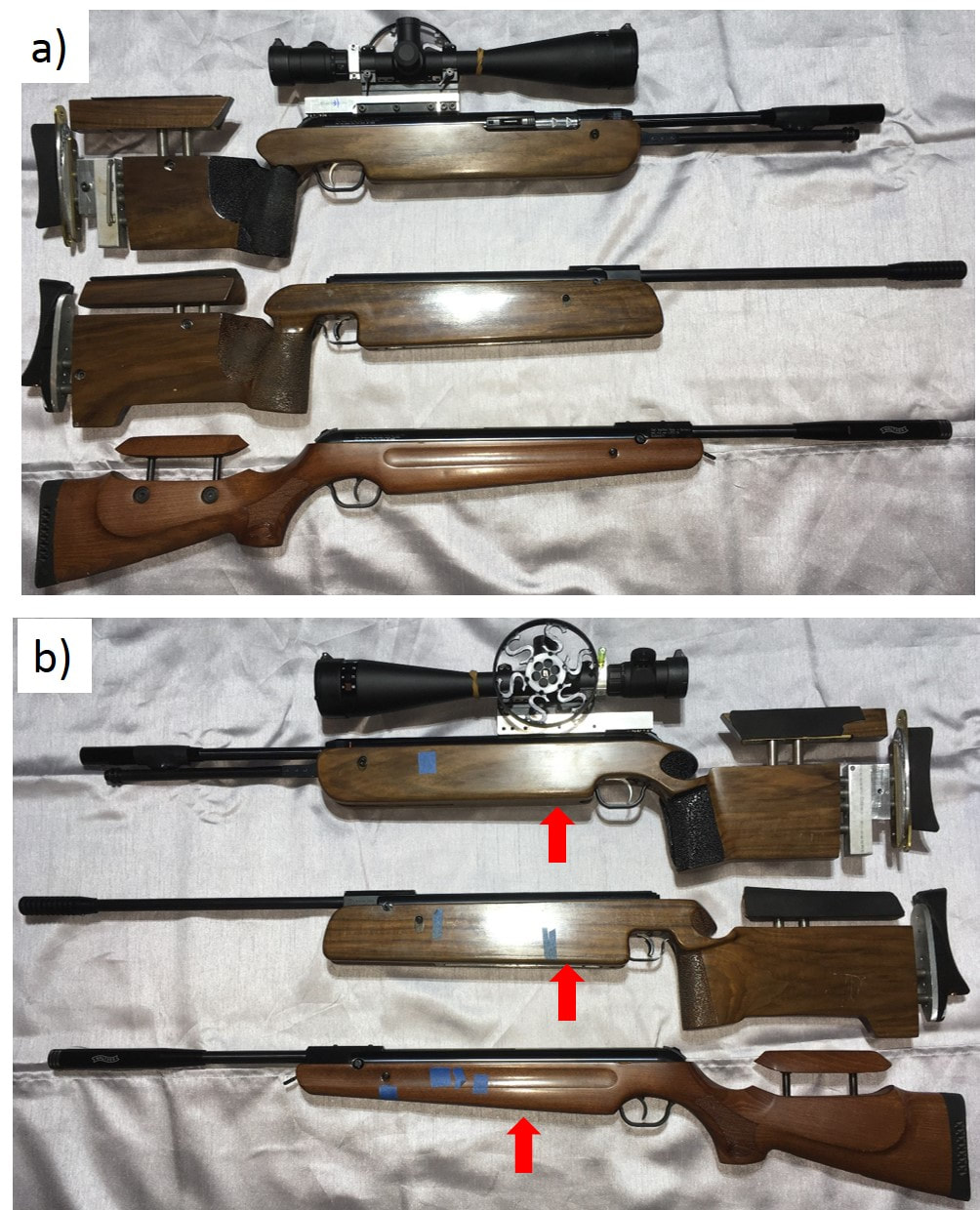
Fig. 2.1 The three protagonists in this story. Top to bottom are the Walther LGU with a Sightron SIIISS1050X60FTIRMOA-H scope, a FWB 124, and a CCA Modified Walther LGV Competition Ultra. All are 0.177” (4.5 mm) caliber. The LGU and FWB 124 stocks are homemade. The aluminum scope raiser block is also homemade. The blue painter’s tape in b) helps to position the forearm optimally and consistently on the front sandbag for benchrest shooting. Red arrows in b) indicate balance points.

All three rifles have been modified, so here’s a brief description of each rifle:

The Walther LGU
Walnut stock is homemade. The receiver is glass-bedded and all the stock screws are pillar-bedded with aluminum tubes. For more info on the stock, please see:

https://www.gatewaytoairguns.org/GTA/index.php?topic=164358.0

I also modified/changed some of the metal parts. The trigger is from Tony Leach:

https://www.airgunforum.co.uk/community/index.php?threads/tony-leach-lgu-trigger-blade.253470/
https://www.airgunnation.com/topic/walther-lgu-lgv-a-new-trigger-option/

I replaced the 15 ft-lb factory spring with a 12 ft-lb Walther LGU spring so that the rifle could be used in World Field Target competitions. I removed the muzzle cap and built a magnetic latch to hold the barrel in place. The original detent barrel latch was hard to use when wearing a shooting mitt and I was concerned that it may have been stressing the barrel. The weight of this rifle with the Sightron scope is 16.3 lbs. The scope with base and rings weighs about 3.4 lbs. For more details on these modifications, please see:

https://www.gatewaytoairguns.org/GTA/index.php?topic=168525.0

The FWB 124 was my first high quality air rifle that I bought in the early 1980’s. I installed the Maccari (Air Rifle Headquarters) Slightly Softer Mainspring kit. I made the stock out of the same walnut blank that was used for my LGU. The reason that there’s an aluminum block at the butt end of the LGU stock is that I didn’t have enough wood left for the LGU after making my FWB 124 stock! The trigger is a Maccari (Air Rifle Headquarters) stainless steel trigger. As with my LGU, the receiver is glass-bedded and all the stock screws are pillar-bedded with aluminum tubes. The weight of this rifle with the Sightron scope is 14.3 lbs. For more background on this rifle, please check out my post on the FWB 300S vs FWB 124 shootout:

https://www.tapatalk.com/groups/yellow/fwb-124-and-fwb-300s-shootout-t239102.html

The Walther LGV belongs to Hector. He custom-tuned it with an anti-bounce piston (ABP). The ABP has a cavity in an enlarged piston stem that holds a non-Newtonian fluid steel. The enlarged stem also functions as a spring guide, it just happens to be inside the piston, not at the rear, as usual. The fluid steel holds a shape (behaves like a solid) when accelerated or under pressure, but when acceleration becomes zero (as when the bounce cycle starts), then the steel becomes fluid again and tries to remain in position by its internal inertia. So the piston is stopped from bouncing and the piston, by holding the position in the compression chamber, maintains the pressure behind the pellet, so that with the same energy input, it can achieve almost 10% more muzzle energy. The weight of this rifle with the Sightron scope is 13.1 lbs.

In Fig. 2.2 I test the accuracy of these rifles at 20 yards. All the shooting was done indoors with the rifles rested on sandbags. In Chapter 3 we will discuss the statistics of group sizes, but I think the key point is that one needs to shoot multiple groups. A single 5-shot, or even a single 10-shot group, doesn’t really say much about accuracy. Maybe it’s just my scientific skepticism, but if someone shows me an amazing 5-shot one-hole group, my first question would be what did the group right before or after that one-holer look like?! With a high quality 50x scope and a solid rest, operator error has been pretty much removed and the group sizes and positions are strictly due to the rifle.

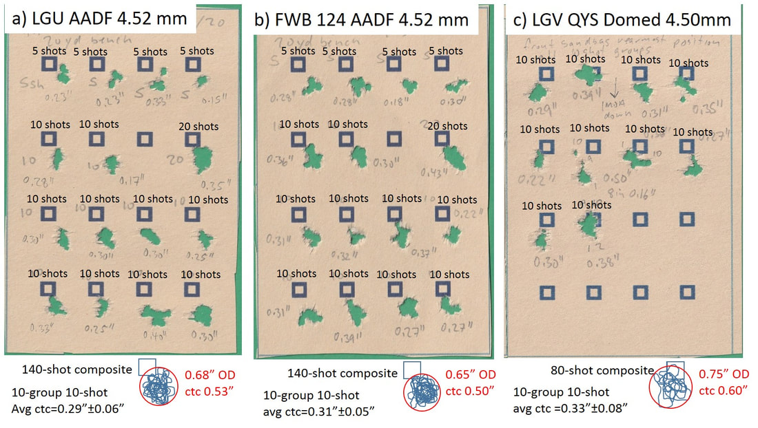
Fig. 2.2 Benchrested groups at 20 yards. For the LGU in a) and FWB 124 in b), there were four 5-shot, two 10-shot, and one 20-shot, followed by eight 10-shot groups. All the groups for the LGV in c) were 10-shot groups.

In Figs. 2.2 a) and b), I shot four 5-shot groups, two 10-shot groups, one 20 shot group, and then eight 10-shot groups with the LGU and FWB 124, respectively. About 20 warm-up shots were taken before the groups were fired for record. The most accurate pellets in my LGU and FWB 124 are the Air Arms Diabolo Field 8.44 gr 4.52 mm. For the LGV in Fig. 2.2c), I only shot 10-shot groups. I tried a few different pellets in Hector’s LGV and found that the Qiang Yuan Sports Domed 8.48 gr 4.50 mm pellets were the most accurate at 20 yards. Group sizes (hand written next to the aiming squares) varied quite a bit even for the 10-shot groups with center-to-center (ctc) distances varying by over a factor of two. The ctc distances were determined by measuring with a caliper the distance between the outer edges of the two most widely separated shots and subtracting the diameter of the hole each pellet makes in the paper (around 0.15”). The averages for ten 10-shot groups was around 0.3” for all three rifles. At the bottom of each target card, I traced out the pellet positions for each target and overlayed them to get composite groups. The composite target for the LGU and FWB 124 contain all 140 shots, which fit inside a circles with diameters under 0.7”. Since I made a scope elevation change for the LGV after the second group, which was destroying my aiming square, I only included the last 80 shots in the composite group. Although the LGV made nice 10-shot groups, the point of impact (POI) tended to drift more (mostly vertically) from group to group than with the other rifles. This is why it’s important to shoot multiple groups in series rather than putting all the shots into a single large groups. It’s hard to see slow drifts in POI in a single 100-shot group! For field target shooting and hunting, what matters most is not the small a 5-shot group a rifle produced, but the size of the kill zone into which a rifle can consistently place all its shots. One key conclusion here is that the 40-year old FWB 124 with its break barrel can hold its own against the latest generation of underlever and breakbarrel air rifles!

I could have simply shown the best groups for these rifles, for example the 0.17” 10-shot group for the LGU, the 0.22” 10-shot group for the FWB 124, and the 0.22” 10-shot group for the LGV, but this would not be telling the whole story and could even be misleading. If the groups were shot outdoors and I had to contend with wind, then it would make more sense to discard bad groups due to wind and focus on the best groups where wind was less of an issue. However, with these tests indoors, there are no external factors except for the rifle itself to blame for larger groups. The best groups here are simply due to luck, where fluctuations in the rifle/pellet system happened to cancel each other out better for one particular string of shots! In most sports, it makes sense to talk about personal bests, so I think we tend to use the best group that a rifle makes to judge its accuracy. However, as we will see in Ch. 3, there is a lot of randomness involved in a single 5-shot or 10-shot group. There is a reasonably good chance (1 in 36) that one could roll the same number three times in a row with a six-sided die, but does that make that die special? Any other die would have the same probability of achieving that remarkable string of rolls!

Figure 2.3 plots the ctc distance for each group. One can clearly see the fluctuations in ctc distances. In Figs. 2.3 a) and b) we can also see how the ctc distance varies with the number of shots in each group for the LGU and FWB 124, respectively. The 5-shot groups tend to be a bit smaller, but not by that much! In a purely random normal distribution (bell curve) one would expect the range of values to increase as one includes more samples. For example, if you measure the height of 20 students in a small classroom, the range of heights you get will be smaller than if you measure the height of 300 students in a large classroom (there’ll be a better chance that some really short and some really tall students can be found in the large classroom). For a normal distribution, this range of values should increase as the square root of the number of samples (in this case the number of student heights measured). Instead of looking at student height, here we are looking at where different shots land on the target. If we include more shots, there’s a better chance that one shot will land farther from the others. However, the group size (analogous to the range of heights in the student example), does not scale as the square root of the number of shots. If that were the case, the 10-shots groups should be 1.4 times bigger than the 5-shot groups (number of shots is twice as large, so we need to multiply the ctc distance by √ 2 = 1.4) and the 20-shot groups should be 1.4 times larger than the 10-shot groups and 2 times larger than the 5-shot groups. It would help if we had a few more 20-shot groups to get a better idea of the average 20-shot group size, but I think it’s clear that were not seeing bell curve scaling of the ctc distance with the number of shots in these groups.

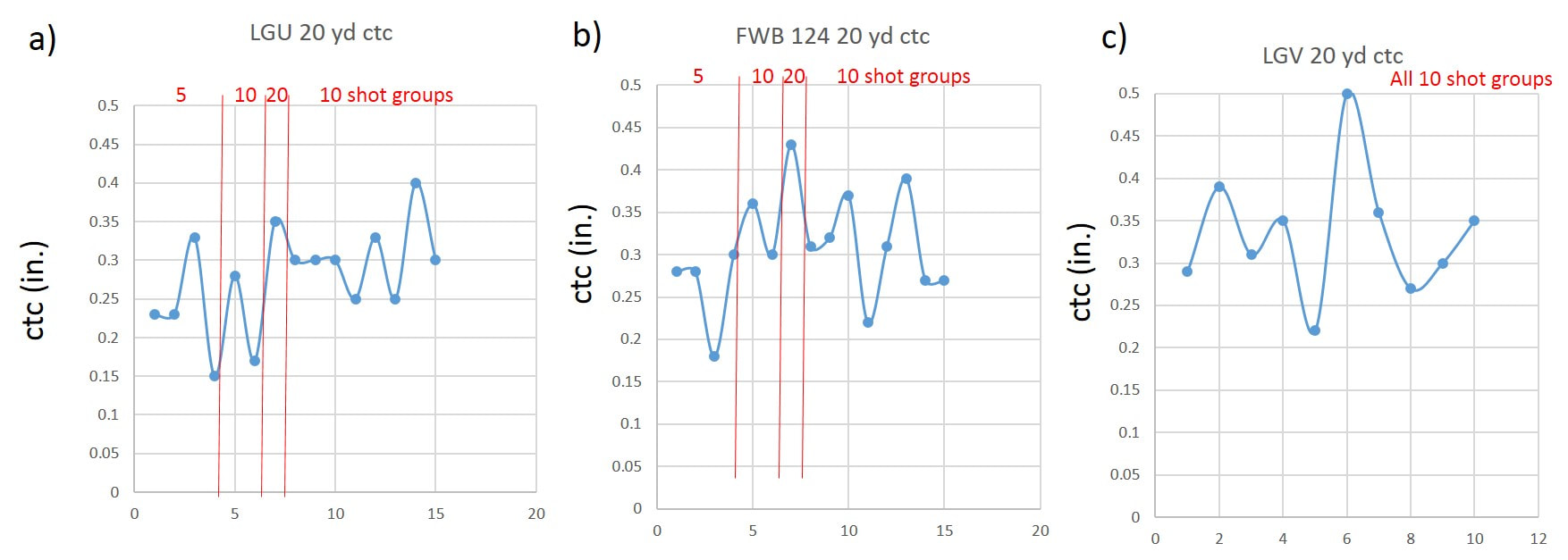
Fig. 2.3 Center-to-center group size for the three rifles benchrested at 20 yards. For the LGU and FWB 124, which had 5-shot, 10-shot, and 20 shot groups, the group size grows with the number of shots in the group, but not as much as one would expect for a perfectly random normal distribution.

In Fig. 2.4, I show how the ctc distance scales with the number of shots in each group. As we already suspected from Fig. 2.3, we see that the ctc distance does not grow as quickly with the number of shots in a group as one might expect from simple bell curve statistics. Instead of growing as the square root of the number of shots x ^ 0.5 (where x is the number of shots and “^” means that we’re taking x to the power of 0.5, which is the same as square root of x), the ctc distance grows as (x ^ 0.36) and (x ^ 0.29) for the FWB 124 and LGU, respectively. This is not too surprising, since there are some constraints on the POI. For example, the pellet will never land behind the shooter no matter how many shots are taken! Although I’m sure that this is commonly known, I couldn’t find a term for it, so I came up with “point of impact envelope” (POIE), that I would like to explore here. I think that every rifle has a POIE in which it will keep all its shots unless something disastrous happens. For example, there may be some side-to-side play in the barrel of a break-barrel springer, but as long as one doesn't loosen the barrel tension screw or hit the barrel to one side with a hammer, the range of possible orientations of the barrel will always be within a certain range and the horizontal spreading of shots due to barrel orientation will be the same whether 10 or 1,000 or 10,000 shots are taken (of course, there may be effects of wear after thousands of shots). So the POIE limits the maximum size of a group as the number of shots goes to infinity. In the example with students’ heights, there is also a height envelope. For example, I don’t think that there are any students taller than 20 feet, so the range of heights is also limited to some extent and does not simply grow forever as the one includes more and more students in the group.

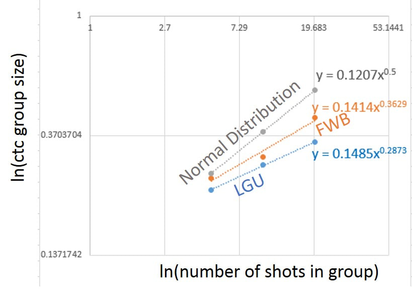
Fig. 2.4 Center-to-center group size scaling with the number of shots per group in a natural log vs natural log plot. For a normal distribution (bell curve), one would expect the ctc group size to scale as the square root of the number of shots (x ^ 0.5), but group sizes for both rifles scale more slowly. In fact, I would expect the group size to saturate at some point (the point of impact envelope), where adding more shots to a group does not cause the group to grow any more, unlike a normal distribution, whose width keeps growing without limit (albeit only as the square root) as the number of samples grows.

Since spring piston airguns generate their own power, the consistency of the powerplant is critical to accuracy. Figure 2.5 shows the muzzle velocity (MV) (in parts a-c) and muzzle energy (in parts d-e) for each shot in the strings shown in Fig. 2.2. The LGU and LGV show a decrease in MV as the rifle warms up. This is probably due to the synthetic piston seal expanding as it warms up, causing more friction between the piston seal and the compression chamber walls and thereby reducing the piston (and pellet) velocity. The MV from the FWB 124, using a factory seal, didn’t change much as the rifle warmed up. Maybe this is an indication of the difference between FWB and Walther piston seals? I also plotted the muzzle energy, which goes as the velocity squared, to look at how the energy that goes into a pellet changes. Later in this chapter, we will talk about the efficiency of these air rifles, so the muzzle energy is probably a better indicator of what the powerplant is doing than the MV. The standard deviations in the MV are fairly high. Some of this can be traced to the pellet. For example, with some tins of AADF and QYS Streamlined pellets in my LGU, I’ve measured MV standard deviations close to 3 fps, but with other pellets I’ve observed MV standard deviations of around 10 fps! Some of it may just be due to the nature of spring piston airguns. My Anschütz 2002 CA PCP match air rifle has MV standard deviations below 2 fps for several brands of pellets. On the other hand, my FWB 300s, which is also a spring piston airgun has MV standard deviations similar to my Anschütz 2002 CA PCP. Of course, the FWB 300S has a steel piston seal and shoots at much lower MV of around 500 fps. Since piston seal friction plays a big role here, the type of lubricant used can be very important. In Ch. 5, we’ll try Krytox in the LGU and FWB 124 to see if it changes MV and if it makes the MV more consistent.

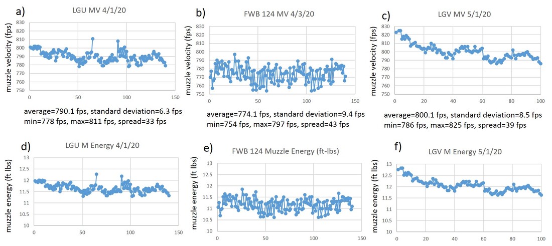
Fig. 2.5 Muzzle velocity a)-c) and muzzle energy d)-f) as a function of shot count for the LGU, FWB 124, and LGV for groups shown in Fig. 2.2.

There is a good chance that a spring-piston air rifle will not always be used off a bench. Since air rifles can be hold-sensitive, it’s important to explore how these rifles do when they are held in different positions. Since I use my air rifles in Field Target (FT) competitions, under WFTF Division rules, it’s critical to test how the rifle shoots from the sitting position, which is used for most shots in an FT match. Figure 2.6a) shows 5-shot groups from these rifles fired from three different positions at 20 yards. I must admit that I was out of practice for this test and my hold was pretty wobbly, but they all were affected by the same lack of practice so the comparison is still valid. The first sitting position, which I’ll call “elbow-top” here, is shown in Fig. 2.6b), where I place my right elbow on top of my right knee while sitting. This position is very stable vertically but does tend to string shots horizontally. Although this position feels pretty stable, it does tend to throw out flyers every now and then. This position doesn’t work very well with my FWB 124 (rifle hold seems more stable, but I get more fliers) and I’ve only been able to use it with my LGU, which is more forgiving of hold variations. The first three targets (from left to right) are from my LGU using the elbow-top hold. The target on the right in the top row is shooting the LGU off sandbags, as was done in Fig. 2.2. The second variation of the sitting position that I use is with my right forearm inside my right knee, which I’ll call “forearm-knee” here. This position may not feel as stable as the elbow-top, but seems to be more consistent. In the second row in Fig. 2.6 a) I shot three 5-shot groups using the forearm-knee position and one 5-shot group off the bench with my FWB 124. In this case, I had better groupings sitting than from the bench, which demonstrates that the FT sitting position can be pretty stable, on a good day! In the third row I repeated the forearm-knee and bench tests using the LGV. In the fourth row I repeated the forearm-knee and bench tests using the LGU. The POI using the two different sitting positions with the LGU (elbow-top in row 1 and forearm-knee in row 3) are quite similar. The forearm-knee position gave slightly tighter groups, with less horizontal stringing. On the lowest circular target, I went back to the elbow-top position with the LGU to compare with earlier target using this position. The POI went up and to the right a bit, but the size of the group was similar to what I found in the first row. In all three rifles, the POI shifted down about 0.5” and a bit to the right when going from sitting to benchrested positions. I have yet to try a 12 ft-lb spring piston air rifle that didn’t exhibit this behavior (ok I’ve only tried three)! The POI in the standing/offhand position (not shown here), tends to be similar to the benchrested POI. It’s ironic that the most stable (benchrested) and least stable (standing) positions have similar POI, with the sitting position, which is between the two in terms of stability, producing a POI that is higher and to the left. For me, the kneeling position (not shown here), has a similar POI as sitting.

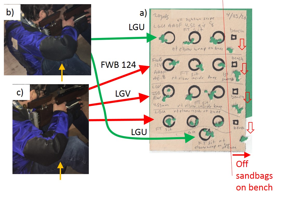
Fig. 2.6 5-shot groups at 20 yards shot from field target sitting position (circular targets) and bench (square targets) in a). Two types of sitting position were used: b) right elbow resting on top of knee and c) right forearm on the inside of knee. All rifles exhibit a similar drop in POI when going from sitting to bench. I had better groupings with the FWB 124 sitting than benchrested!

Since the shift in POI in going from the benchrest to the sitting position seems to be very robust and universal, I did some further testing to figure out what causes this shift. I typically shoot the benchrested position using the artillery hold, with no contact between the rifle buttpad and my shoulder. The rifle is held very lightly and allowed to recoil as freely as possible on the sandbags. In the sitting, kneeling, and standing positions, the rifle buttpad is in firm contact with my shoulder. I’ve noticed that when I pulled the rifle tighter against my shoulder in the sitting position, the POI went up (maybe this is what happened in the last target from the sitting position at the bottom of Fig. 2.6a?), so in Fig. 2.7, I tested the effects of shoulder pressure on POI. In Fig. 2.7, I shot the LGU at 20 yards from four different positions. A: benchrested, artillery hold with no contact between shoulder and buttpad; B: benchrested with buttpad pulled against shoulder; C: elbow-top sitting (see Fig. 2.3b); D: forearm-knee sitting (see Fig. 2.3c). Again, we see that the POI shifts up and left when going from artillery-hold benchested (A) to the sitting positions (C and D). Lots of things change when going from the benchrested to sitting positions, so in position B, the only thing I changed was pulling the rifle against my right shoulder. Everything else was the same as in the benchrested artillery-hold position (A). Although there are some variations in the difference between the POI of the artillery-hold benchrested (A) and the shoulder contact benchrested (B) positions, the POI for B was consistently higher than for A. Of course the POI for the sitting positions (C and D) was even higher. It’s not clear to me whether this is due to barrel harmonics changing with the shoulder pressure, or whether the rifle tends to rotate upward due to the shoulder pushing against the recoiling rifle. Since this effect is seen in all three rifles, I tend to think that the rotation explanation works better since it should be similar in all three rifles whereas barrel harmonics could be very different among the three rifles. However, it’s clear that shoulder pressure is a dominant cause of the higher POI.

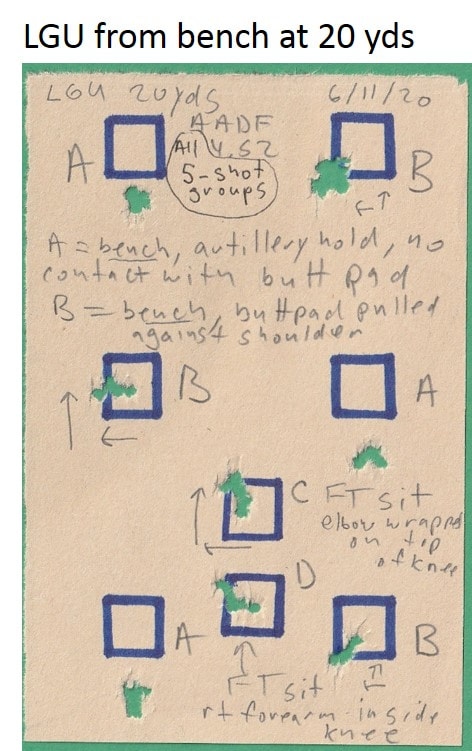
Fig. 2.7 5-shot groups with the LGU at 20 yards shot from four different positions. A: bench, artillery hold with no contact between shoulder and buttpad; B: bench with buttpad pulled against shoulder; C: FT sitting with right elbow wrapped around/resting on top of right knee (see Fig. 2.3b); and D: FT sitting with right forearm inside right knee (see Fig. 2.3c). Buttpad contact on shoulder causes POI to shift up and left, no matter what position is used.

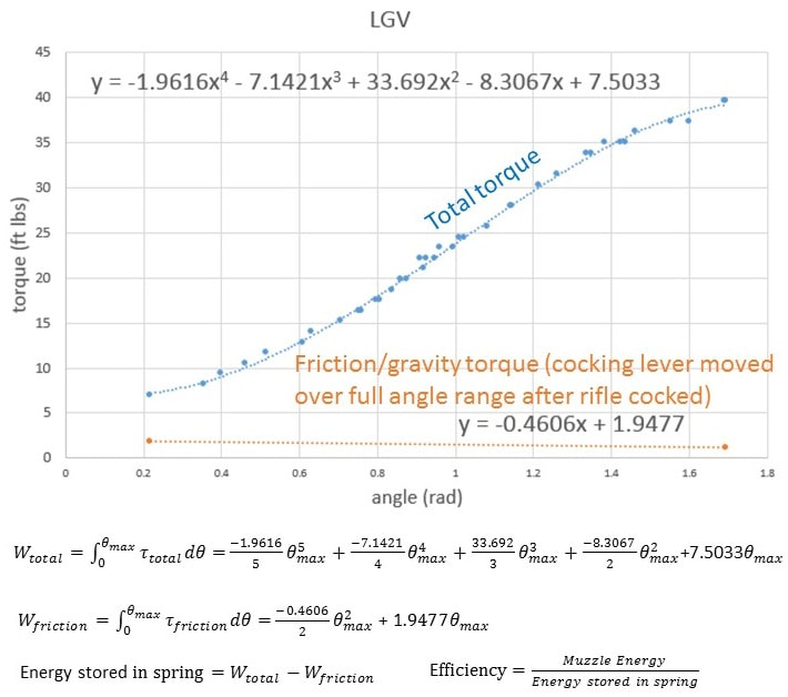
In Fig. 2.2, we saw that the veteran FWB 124 was very competitive in terms of accuracy, but how does it compare in terms of efficiency with the LGV and LGU, that use the latest in materials and design? Although the LGU and LGV use the same spring and piston, the LGV transfer port (TP) is offset and is much longer. How do the LGV and LGU efficiencies compare? In Fig. 2.8, I look at the work required to cock these three rifles. The cocking force vs barrel/lever angle look very similar, with the characteristic s-shaped curve that we discussed in Ch. 1.

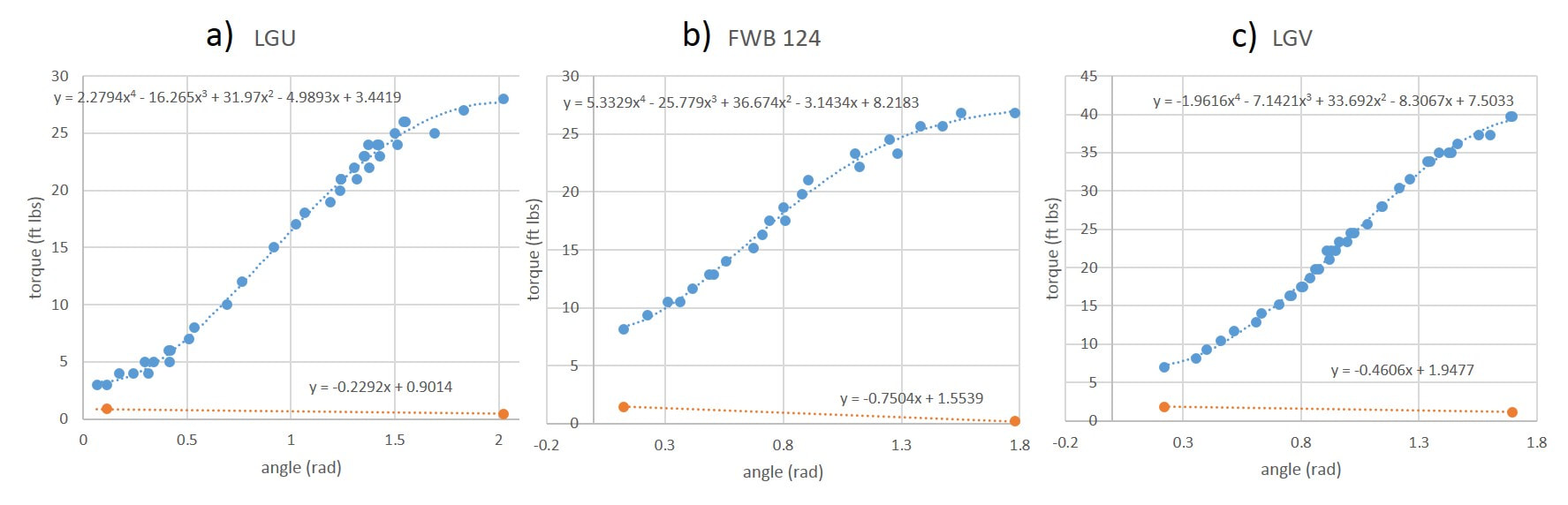
Fig. 2.8 Torque as a function of cocking lever/barrel angle for the a) LGU, b) FWB 124, and c) LGV. By integrating the curves (areas under the curves) one can obtain the total work to cock the rifles. By subtracting the work lost to friction and gravity (initially the barrel must be lifted) one can estimate the energy stored in the spring. Dividing the muzzle energy by the energy stored in the spring determines the efficiency of the rifle.

If we compare the work that goes into cocking the spring (Fig. 2.8) with the energy that comes out with the pellet, we can obtain the efficiency of a spring piston air rifle. The efficiencies of the three rifles are shown in Fig. 2.9. Maybe here one can see the age of the FWB 124’s design, with the lowest (but still pretty good) efficiency? Surprisingly, the LGV with its long TP had efficiencies with JSB Exact and QYS Dome pellets that were very close to the LGU. In fact the LGV did a little better than the LGU with the JSB Exacts. The LGU with its short, central TP had the highest efficiencies and did well with all the pellets. It’s hard to speak of overall efficiency, since there was a lot of variation in muzzle energy (and therefore efficiency) with different kinds of pellets. The main takeaway here is that the LGV with its long non-central TP is pretty much just as efficient as the LGU with its short central TP! This may be due to the 10% gain in muzzle energy from the anti-bounce piston, so in Chapter 4, we’ll take another look at the efficiencies of the LGU and LGV with swapped pistons and mainsprings.

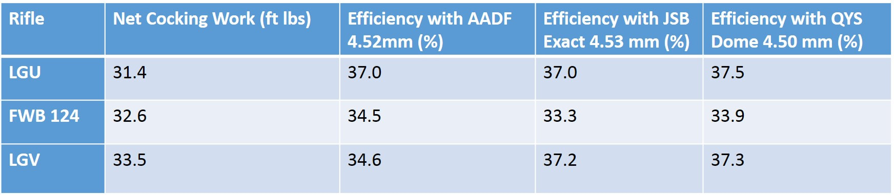
Fig. 2.9 Efficiency of the LGU, FWB 124 and LGV with various pellets.

Another important factor in helping us get the most accuracy out of an air rifle is the trigger pull. All three of the rifles had modified triggers. I installed a replacement trigger from Tony Leach in my LGU. The tips of the set screws were originally polished to a fairly fine point, which allows more precise leverage, but I rounded these to a larger radius of curvature to make sure that they don’t scratch the bottom sear. Photos and a more detailed description can be found at:

https://www.gatewaytoairguns.org/GTA/index.php?topic=168525.0

This is a wonderful two stage trigger that comes pretty close to the light weight and crispness of the triggers on my Anschütz 2002CA and FWB 300S! This trigger changed the way I shoot at FT matches. I simply let the rifle sit where it wants and can pull the trigger without moving the rifle off target.

Hector modified his LGV trigger by adding longer adjustment set screws. The trigger pull is a bit heavier than the Leach trigger, but it is more than light and crisp enough for a clean trigger pull that doesn’t disturb one’s aim. Photos and a more detailed description can be found at:

https://www.ctcustomairguns.com/hectors-airgun-blog/a-yankee-tune-for-the-walther-lgu

Unfortunately, the FWB 124 doesn’t have the multilever lever arrangement with adjustable engagement points like the LGV and LGU, which use the same trigger and are very similar in design to the Weihrauch Rekord and Air Arms TX 200 triggers. However, with careful honing of the engagement surfaces and adjusting the pull weight screw so that one just barely feels the second stage engage, one can get a pretty good trigger pull in the FWB 124. I had a hard time figuring out how the FWB 124 trigger works and found the article below to be very helpful:

https://forum.vintageairgunsgallery.com/feinwerkbau-rifles/feinwerkbau-modell-124/

In my FWB 124 I replaced the factory aluminum trigger blade with a solid stainless steel trigger blade from Jim Maccari at Air Rifle Headquarters. I could feel the original aluminum trigger flex as the shot was about to be released, but that’s not a problem with the beefy stainless steel trigger. One can lower the pull weight by backing the adjustment screw out to the point that one loses the second stage, but this results in a long (albeit fairly light) pull with no hint of when the rifle will fire. By screwing in the adjustment screw until one can just barely feel the second stage engage, one can get a very predictable two-stage pull. On my FWB 124, the trigger feels like it snaps into a position as the second stage engages, and then it takes only a bit more pressure to release the shot.

Figure 2.10 shows the trigger pull weight for 10 shots with the a) LGU, b) FWB 124, and c) LGV. The light pull weights on the LGV and LGU make them easier to shoot accurately, but the FWB 124 trigger also works great. The pull weights are also quite consistent.

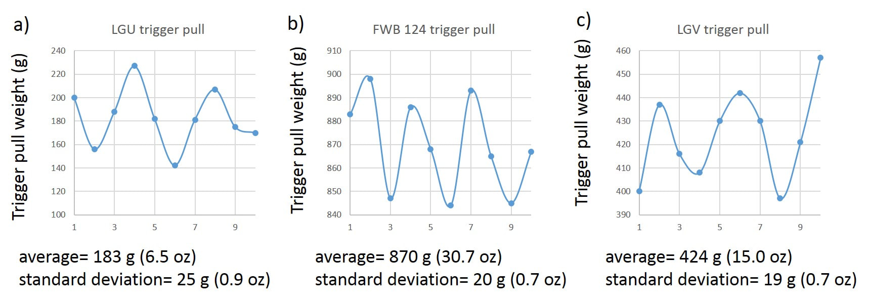
Fig. 2.10 Trigger pull weight for ten shots for the a) LGU, b) FWB 124, and c) LGV.

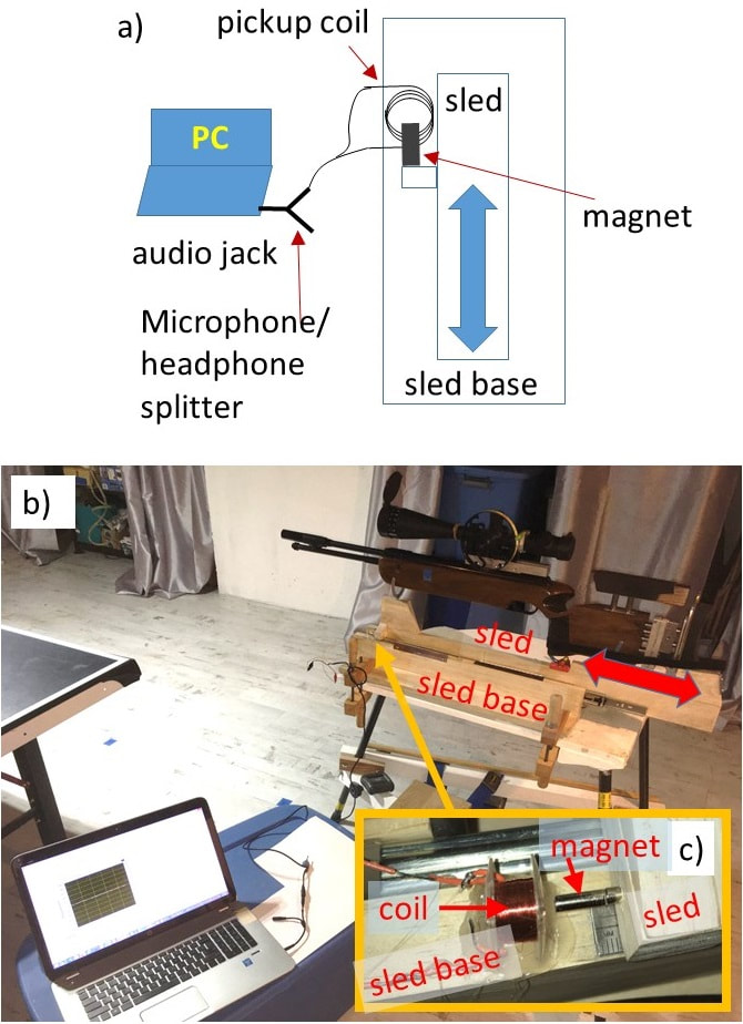
We finish this chapter by looking at how the three rifles recoil using the dynamograph. There is some universal behavior in the recoil of all three rifles, but there are also some interesting differences. Figure 2.11 shows the position, velocity, and acceleration as functions of time for all three rifles. It’s important to remember that the LGU and FWB 124 with their target stocks weigh about 2 to 3 pounds more than the LGV. The pickup coil measures the sled/rifle velocity, which is plotted in red, and then we use calculus to determine the position and acceleration of the rifle from the measured velocity. All three rifles initially recoil backwards (negative velocity) as the piston accelerates forward at the start of the shot. Approximately 10 ms later, the piston starts moving backward, causing the rifle to move forward (positive velocity). The ratios of the forward peak velocity to the backward peak velocity are remarkably similar, with values of 0.52, 0.50, and 0.54 for the LGU, FWB 124, and LGV, respectively. The peak forward and backward velocities for the LGU (-700 mm/s backward and 365 mm/s forward) and FWB 124 (-700 mm/s backward and 350 mm/s forward) are very similar. The velocities of all three rifles oscillate at longer times, but the FWB 124 shows a distinctive higher frequency ringing (wiggles). This is probably due to the loose fitting metal spring guide that allows the spring to buzz after the shot. The spring guide and top hat in the LGU fit the spring very tightly, which greatly reduces spring vibrations. In the LGU and FWB 124, the spring and piston are nearly dry, with only a very light coating of moly and Superlube. On the other hand, the LGV mainspring is coated with spring tar. It’s also informative to look at the acceleration as a function of time. Remember, acceleration tells us how fast the velocity is changing. In all three rifles, the initial dip in backward acceleration is smaller than the first peak in forward acceleration, which suggests that the spring initially pushes the piston forward more gently causing it to pick up speed more slowly compared to the more abrupt stopping of the piston’s forward motion and bounce toward the rear when it reaches the front of the compression chamber. Qualitatively, the traces for the LGU and LGV look very similar, with the main quantitative difference probably coming from the difference in the weight of the two rifles. In addition to the higher frequency ringing, the FWB 124 also shows a very large and sharp backward acceleration spike at around 0.018 s. Maybe this is the piston bouncing hard forward after the rearward surge?

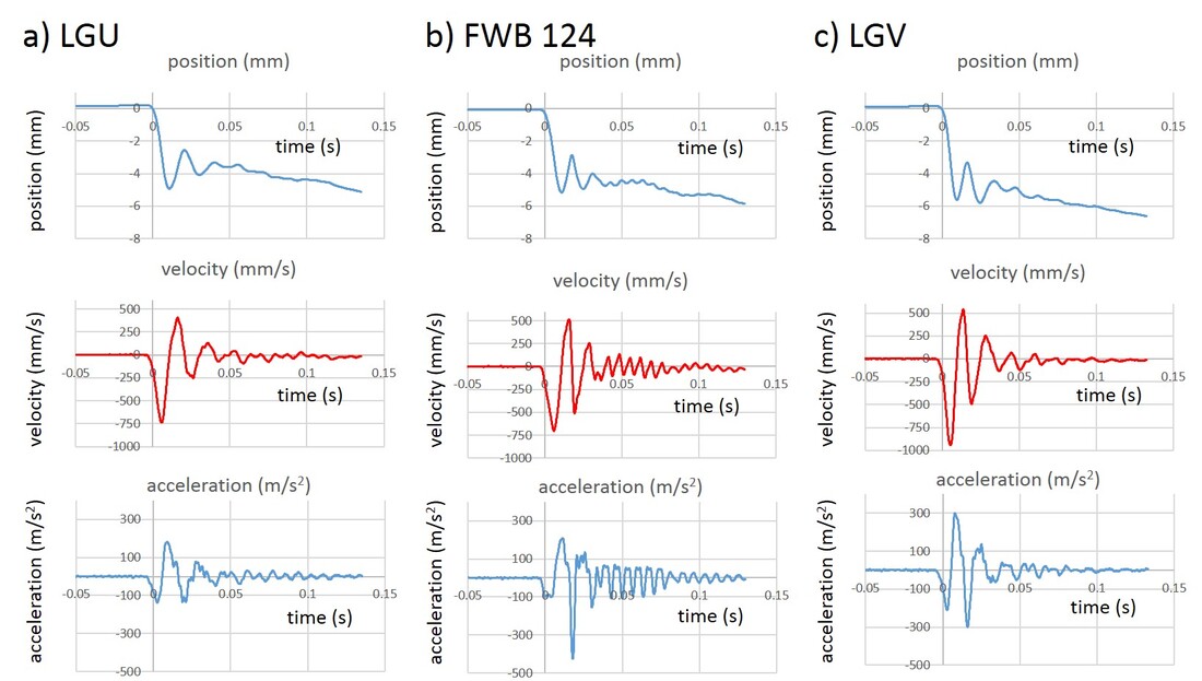
Fig. 2.11 Recoil traces showing the position, velocity, and acceleration of the sled-mounted rifle over 250 ms for the a) LGU, b) FWB 124, and c) LGV. Note that the rifles first move backward (velocity and acceleration are negative), but then the rifles surge forward as the piston stops and starts moving backward. This is followed by oscillations. The net overall movement of all three rifles is backward.

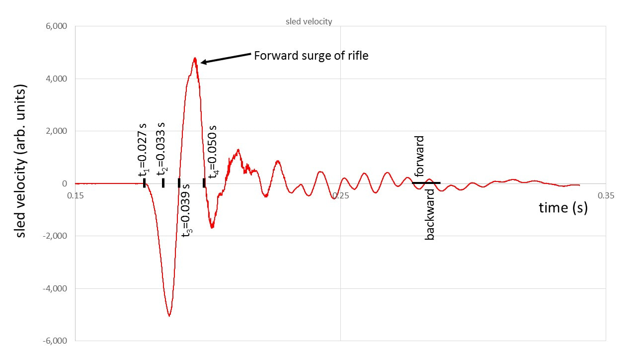
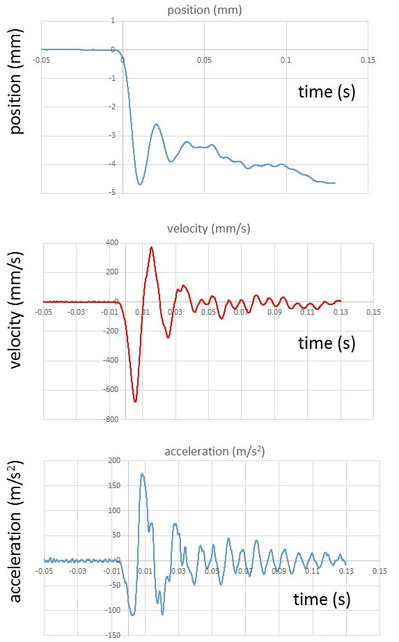
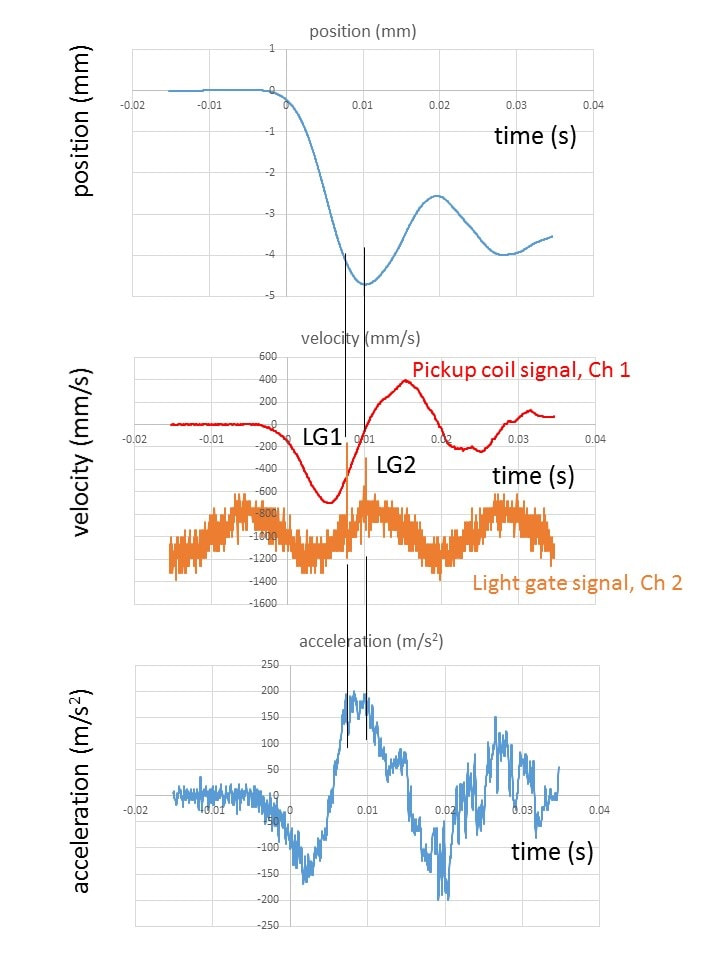
Since the pellet leaves the barrel in less than 12 ms, only the initial recoil will affect accuracy, so in Fig. 2.12, I’ve zoomed in on the first part of the recoil. I’ve also included the light gate signal so that we can see when the pellet leaves the barrel. In all three rifles, the pellet leaves the barrel at the peak forward acceleration of the rifle, when the piston is still moving forward but is slowing down the most rapidly on the cushion of compressed air that is ahead of it. The time from the start of the recoil motion to when the pellet leaves the barrel (first spike in light gate signal orange trace, indicated by vertical red lines) is very similar for all three rifles. It’s between 10 and 11 ms. Remember, that a pellet traveling 800 fps covers 1” in about 0.1ms, so differences in barrel length will also affect this time. It’s also hard to determine precisely when the rifle started moving backward since the initial rearward motion starts gradually.
I recently built a system to measure Pellet Dwell Time (time from trigger pull to pellet leaving the muzzle). I placed a contact microphone on the receiver tube near the trigger, which picks up the sound of the sear tripping. The signal from the microphone is sent to one of the channels on the oscilloscope, and the other channel records the light gate signal, allowing the time between sear release and pellet exit to be measured. This setup is too new to be included in this series, but I hope to post the results someday soon.
Now one can see more clearly that the initial backward acceleration of all three rifles is smaller than the forward acceleration when the piston bounces, which is consistent with the picture of the initial gradual push that the spring imparts on the piston and the more abrupt bounce of the piston backward when it reaches the front end of the compression chamber. One dramatic difference is that the first dip in the backward acceleration of the FWB 124 (-130 m/s²) is significantly smaller in magnitude compared to the dips in the backward accelerations of the LGU (-150 m/s²) and LGV (-244 m/s²). I think that this is due to the longer and softer spring in the FWB 124 compared to the shorter and stiffer springs in the LGV and LGU. The preload in the FWB 124 is around 1.5” while the LGU and LGV have only about 1” of preload. Since the LGV and LGU get more energy out of their springs with less preload than the FWB 124, they must have stiffer springs. It would be very interesting to see what longer and softer mainsprings in the LGU and LGV would do to their recoil cycles. I agree with Jim Tyler in his July 2018 Airgun World column, that softer springs with more preload can soften piston bounce and improve accuracy. Although the reduction in backward acceleration of the FWB 124 is consistent with a softer spring, it doesn’t look like the peak positive acceleration at the piston bounce is reduced that much compared to the LGU. To test this, we really should try different springs and preloads in the same rifle, rather than comparing different rifles with different preloads. When the piston bounces back, the rifle moves forward and one gets a peak in the rifle velocity in the red traces in Fig. 2.12. According to that peak, the anti-bounce piston mechanism does not appear to be significantly decreasing the piston bounce in the LGV compared to the LGU and FWB 124.
On the other hand, since the pellet has left the rifle before the rifle starts moving forward, maybe we shouldn’t be so concerned with piston bounce, at least as far as accuracy is concerned? Of course, it would be much better to try a regular piston in the same LGV rifle and compare it to the ABP results, rather than comparing with other rifles. We’ll take another look at this in Ch. 4. Now that we have the capability to record the recoil traces with sub-ms time resolution, we can see with great detail what tuning is doing to the recoil cycle!

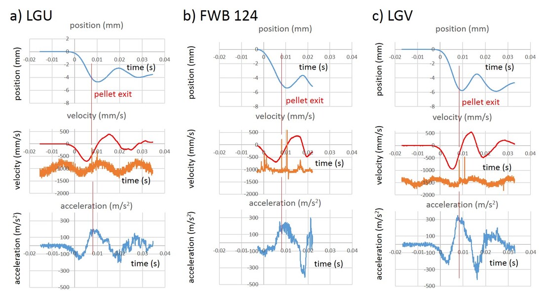
Fig. 2.12 Recoil traces showing the position, velocity, and acceleration of the sled-mounted rifle zoomed into a 50 ms window for the a) LGU, b) FWB 124, and c) LGV. The lower, orange traces plotted in the middle velocity panels show the light gate signals, with the first pulse occurring when the pellet is about 2” in front of the muzzle (vertical red lines) and the second pulse occurring when the pellet passes the second light gate, approximately 25” in front of the muzzle.

2 Comments

Shot cycle Dynamics in 3 Spring-Piston Airguns Chap 1

4/15/2021

9 Comments

Diagnostic Equipment:
How can we understand better what our air rifles are doing?

Spring piston air rifles are deceptively simple. They “just” use a spring to drive a piston down a compression chamber and that compressed air drives a pellet out of the barrel and towards the target.

However, in the roughly 10 milliseconds (ms) it takes for the pellet to leave the barrel, the air in the compression chamber reaches over of 1,200 °F and 900 PSI when the piston reaches about 95% of its stroke (adiabatic compression), the rifle recoils back, but then starts to move forward as the piston stops its forward motion and bounces backward. To understand what is going on involves mechanics (spring energy, kinetic energy, friction, etc.) as well as thermodynamics of a compressible fluid. This is what makes spring piston air rifles so fascinating, fun and, at times, frustrating!

In an effort to better understand what is going on with spring piston air rifles, Hector Medina suggested that we work together on some basic tests of three spring piston air rifles (Walther LGU, Walther LGV, and a FWB 124). I have really enjoyed working with him on this journey and we are also grateful to Willem Laan for his support and helpful questions and suggestions. Since many discoveries begin with good questions, the chapter titles are simple questions. We began with just a few questions, but as you will see, the number of chapters grew to NINE!

So let’s take a closer look at how we can use various diagnostic tools to better understand our air rifles.

The simplest, and probably the most important tool, consists of a piece of paper with an aiming point drawn on it! In the end, the most important criterion for any air rifle is how well it can place its shots on a target. Lots of power is useless without accuracy. The famous gun writer Col. Townsend Whelen once said that “Only accurate rifles are interesting.” So you’ll see lots of shots on targets in these blog entries and I hope that you’ll find the rifles that we tested “interesting.” But the targets don’t always tell you why a rifle is shooting well or poorly, so we need to use other diagnostic tools.

Chronograph

One of the first diagnostic tools that is readily available is a chronograph, which gives the muzzle velocity of the pellet. By placing the chronograph at different distances from the muzzle one also can determine how quickly the pellet is slowing down, which gives us the ballistic coefficient (BC) of the pellet-rifle combination. The BC lets us model the trajectory of the pellet better and tells us how well the pellet handles wind; high BC pellets do much better than low BC pellets in windy conditions. Commercial chronographs are available for under $100 (be sure to get LED lights for indoor shooting) or you can make your own for a few dollars, as I did. I used scrap wood and wire and only had to spend a few bucks on infrared LEDs and photodiodes. The Softchrono app (the software can be downloaded here), which was originally designed to use the sound of the rifle firing and the pellet hitting the target to obtain muzzle velocity can be easily adapted to use the signals from the LED/photodiode light gates going into a computer’s audio jack to measure pellet velocity. The nice thing about using infrared LEDs and photodiodes in this DIY chronograph is that one doesn’t have to worry about visible light coming from different places messing up the light gate signals. For more details, please see this thread (my chrono is described in post #6):

https://www.tapatalk.com/groups/yellow/viewtopic.php?p=1899493#p1899493

For the original Poor Man's Electronic Chronograph post, with more details on the audio jack circuit, as well as the infrared LEDs and photodiodes, please check:

https://www.tapatalk.com/groups/yellow/poor-man-s-electronic-chronograph-t186868.html

A chronograph is especially important in spring piston air rifles, because the muzzle velocity (and especially changes in MV) can be a symptom of bad seals, poor/old lubrication, weakening mainspring, poor/irregular fit of pellets in bore, dirty bore, etc.

Recoiloscope

One of the most critical aspects of spring piston air rifles is that the pellet’s point of impact (POI) depends much more on how the rifle is held than for most kinds of other rifles (pneumatic air rifles and powder burners). This is called hold sensitivity, and a good way to study this is to see how the air rifle moves at firing. To measure the rifle’s backward/forward motion on firing, I’ve borrowed an excellent recoil sled that was designed and built by Steve Herr (aka Nitrocrushr on GTA), who was kind enough to send us these photos and diagram.

Fig. 1.1 Dimensioned build diagram of Steve Herr’s recoil sled.

Figure 1.2 shows a photo of an air rifle mounted on the sled. The rifle is supported on the sled by u-shaped vinyl-coated hooks (labelled 1 in Fig 1.2) under the forearm and under the stock near the buttplate. A long hook and loop strap (labelled 2 in Fig 1.2) is wrapped around the pistol grip or through the back of the trigger guard to pull the rifle tight against a vertical stop at the back of the sled. The sled itself is held onto the base by ball-bearing drawer slides. There is very little friction in moving the sled back and forth. A ruler (labelled 3 in Fig 1.2) is placed on the base next to the sled to measure sled position. Bubble levels (labelled 4 in Fig 1.2) make sure that the sled is level side-to-side and front-to-back. Finally an air bladder (labelled 5 in Fig 1.2) from a blood pressure cuff is used to depress trigger without moving the rifle. Very clever idea Steve!

Fig. 1.2 Steve Herr’s recoil sled with rifle attached. Also visible are 1) u-shaped supports, 2) hook and loop strap, 3) ruler to measure sled position, 4) bubble levels and 5) air bladder to depress trigger without moving the rifle.

For more info on the sled, please see:
https://www.gatewaytoairguns.org/GTA/index.php?topic=160511.msg155787786#msg155787786

Figure 1.3 shows how I used the sled to make recoil measurements. For the short distances travelled (~6mm=0.25”) and the short times (10's of milliseconds), the friction of the sled has a negligible impact on the energy and momentum of the recoiling rifle. In fact, one probably could get away with just resting the rifle on sandbags, but the sled makes the recoil measurements much easier, more repeatable, and more accurate. One complication that the sled adds is that the sled itself, which moves with the rifle, weighs 2.4 lbs. This added weight to the rifle will affect its recoil a bit.

Fig. 1.3 Our recoiloscope: Recoil trace measurement using a the sound card on laptop PC. a) setup schematic, b) setup photo, and c) close-up photo of magnet and coil. The magnet moves with the sled as rifle recoils and the coil is stationary on the sled base.

So what do we measure with the sled? The first thing one can do is take a video of the recoiling rifle. Steve placed an indicator on the sled that points to the ruler on the sled base, so one can see the position of the sled as a function of time. Most smartphones have a high speed video setting with a frame rate of 240 frames per second. This gives a time resolution of just over 4 ms that can capture the recoil motion reasonably well.
Below are some videos that I took of the LGV, LGU, and FWB 124 fired on Steve’s sled.
Make sure you select the lowest play-back speed (0.25X).

LGV recoil video:
https://youtu.be/rh9VVykKKiM
LGU recoil video:
https://youtu.be/ynzrbddtN1U
FWB 124 recoil video:
https://youtu.be/2RKUY3x48zE

These videos give a good qualitative picture of how the rifle is recoiling and one can clearly see the forward surge after the initial backwards recoil, as well as the later oscillations. However, the poor time and spatial resolution make it hard to study the recoil in detail. To get more accurate sled position data with better time resolution, I built an inductive pickup coil system that measures the velocity of the sled with respect to the sled base. As can be seen in the diagram in Fig. 1.3a), I attached a permanent magnet (neodymium-iron- boron rare earth magnet) to the sled that moves with respect to a wire coil that is attached to the sled base. The motion of the magnet with respect to the base produces a voltage in the coil that can be recorded as a function of time with an oscilloscope. In this case I used a soundcard on my laptop computer to record the signal (pc oscilloscope) and later we’ll use some stand-alone oscilloscopes. The voltage is proportional to the velocity of the magnet, so we can measure the rifle/sled velocity during recoil with a sub-millisecond time resolution. A photo of the system is shown in Fig. 1.3b) and a close-up photo of the magnet/pickup coil is shown in Fig. 1.3c).

The basic physical principle that allows this system to measure the sled velocity is Faraday’s law of induction, which basically says that an electrical current will be induced in a coil of wire if the magnetic field, going through the area bound by that coil, changes. As the sled moves back and the permanent magnet moves away from the coil, the amount of magnetic field going through the coil decreases, and a voltage will be induced in the coil that produces an electrical current to try to replace that lost magnetic field.

Electrical currents in coils produce magnetic fields, so the induced currents can actually replace some of the lost magnetic field as the permanent magnet moves away from the coil. The change in magnetic field at the coil is directly proportional to how fast the magnet is moving away from, or towards, the coil, so the coil voltage is proportional to the velocity of the magnet/sled. I made the coil by winding exceptionally fine magnet wire (OD about 0.002”) around a sewing machine bobbin (I did get permission from my wife to steal one of her bobbins!). I mounted the bobbin on a dowel, which I then spun on a power drill. I lost track of the number of turns after about 100, and went until the wire broke. I got roughly the first third of the bobbin wound with wire. The more turns of wire in the coil, the more sensitive the system will be.

Since the system allows one to see the rifle’s recoil and since the signal is picked up with an oscilloscope, we like to call it the “recoiloscope.” A schematic of the recoiloscope is shown in Fig. 1.3a). One can use the audio jack on a computer and oscilloscope software to read the coil voltage (and thereby the sled velocity) as a function of time. I wrote my own data-taking program using National Instrument’s LabView, but there are lots of sound card oscilloscope programs that you could use. I’ve also used Soundcard Scope (https://www.zeitnitz.eu/scope_en), which is free but unfortunately doesn’t allow you to save the data.
Figure 1.3b) shows a photo of the setup, including the customized Walther LGU that was used for all the tests in this chapter. More info on the rifle can be found at:

https://www.gatewaytoairguns.org/GTA/index.php?topic=168525.0

It’s important to mention that this system was inspired by Jim Tyler, who developed an electrical “recoilometer.” His monthly Technical Airgun column in Airgun World magazine is brilliant and full of deep insights into the finer inner workings of spring piston airguns. Although Jim does not give much technical detail on his recoilometer, I’m assuming it operates using a pick-up coil system as well.

Figure 1.4 shows a typical recoil trace from a Walther LGU measured using the recoiloscope from Fig. 1.3. The vertical axis in the plot in Fig. 1.4 is the coil voltage, which is proportional to the sled/rifle velocity, and the horizontal axis is time in seconds. Positive voltages correspond to the rifle moving forward and negative voltages mean the rifle is moving backward.

Fig. 1.4 Recoil trace using the recoiloscope with a laptop PC. t1 is when the rifle starts recoiling backwards. t2 is when the rifle reaches the maximum rearward velocity and starts slowing down it rearward motion. t3 is when the rifles starts to surge forward. t4 is when the rifle starts going backward again and begins smaller oscillations backward and forward.

Unlike a firearm, where the recoil is strictly backward, a spring piston airgun exhibits a strong forward surge as the piston slows down/stops at the front end of its travel. One way to think of it is that the rifle must apply a backwards force to the piston to stop it, and therefore, by Newton’s third law, the piston must be pushing the rifle forward with the same magnitude force.

In Fig. 1.4, several key times are identified. When the trigger is pulled and the piston accelerates forward, the rifle starts to recoil backward at time t1. About 6 ms later, at time t2, the rifle reaches the maximum rearward velocity and starts slowing down its rearward motion. It’s still going backwards, but is slowing down. At time t3, 12 ms after the start of the recoil, the piston slows down and the rifle starts to surge forward. At time t4, 23 ms after the start of the recoil, rifle recoils backward again and begins smaller oscillations backward and forward. I think that these smaller oscillations are caused by coils in the mainspring vibrating back and forth.

Dynamograph

Since the pellet is disturbed by the motion of the rifle only while the pellet is in the barrel, a key question is:
When does the pellet leave the barrel? To measure the pellet exit time, I combined the recoiloscope with the homemade chronograph that I mentioned earlier in this chapter. We call this system a “dynamograph.”

The DIY chronograph requires a laptop pc (to power the infrared LEDs and the light gate circuit). I borrowed a two-channel digital storage scope (Tektronix TDS 2024B) to simultaneously measure the pickup coil signal (sled velocity) and the light gate signal (when pellet crosses under the light gates in the DIY chronograph). The oscilloscope doesn’t have to be anything special. The main features are that it can record two channels at the same time, has a time resolution of 0.1 ms or faster, and can save the data so that we can analyze and plot the traces. As we’ll see later, it’s helpful to have an oscilloscope that can do dc as well as ac input coupling. At the end of the discussion of the dynamograph, I will test a $100 mini USB oscilloscope and show that it can work as well as the Tektronix oscilloscope.

Figure 1.5a) shows a schematic of the dynamograph. The recoil velocity measurement is the same as before except that now the pickup coil signal goes to channel 1 of the oscilloscope instead of the sound card on a PC. The oscilloscope measures the pickup coil voltage, which tells us about the sled velocity, and the light gate signal from the DIY chronograph, which tells when the pellet crosses the light gates in front of the muzzle. The PC now only serves to power the LEDs of the light gate through its USB port and to power the photodiode detectors in the light gate circuit through the audio jack port. The pickup coil voltage goes to channel 1 on the oscilloscope and the light gate voltage (two new wires are connected to the original light gate circuit) goes to channel 2. This allows us to record the sled velocity and the pellet crossing the light gates at the same time.

The DIY chronograph is connected to the PC the same way as it was for use as a chronograph except that the two wires (blue wires going to Ch. 2 of oscilloscope in Fig. 1.5a) are connected to the light gate circuit going to the PC’s audio jack (black wires in Fig. 1.5a). One of the wires connects before the first light gate and the other one connects after the second light gate, so we’re measuring the voltage across the entire photodiode circuit. When the pellet goes through a light gate, it blocks the light from the infrared LED at the top of the gate from going to the photodiodes (detectors) at the bottom of the gate, which causes a positive voltage spike in the photodiode circuit.

Fig. 1.5 Our dynamograph records the recoil velocity and pellet exit signal using an oscilloscope and DIY chronograph. a) setup schematic and b) setup photo.

As mentioned before, the dynamograph records the velocity of the sled as a function of time on Ch. 1 on the oscilloscope, while on Ch. 2 we can see when the pellet leaves the muzzle, passing light gate 1 and when it passes the second light gate, which is 1.88 ft after the first light gate. The time separation between the light gate pulses gives us the pellet’s velocity, whereas the first light gate pulse gives us the time when the pellet left the barrel, and is no longer affected by rifle vibration/motion. Since LG1 is not exactly at the muzzle but is located about six inches away from it, the LG1 pulse occurs about 0.6 ms after the pellet leaves the barrel (assuming a pellet velocity around 800 fps), but that’s close enough for the time scales that we’re looking at. From now on, we’ll just treat the LG1 pulse as the time the pellet leaves the barrel, but if you wanted to be super accurate, you could subtract 0.6 ms to get the actual time the pellet leaves the muzzle.
Figure 1.5b) shows a photo of the dynamograph setup, again with my trusty LGU. The light gates are labeled in the photo. You can see how the DIY chronograph is connected to the PC (USB port and audio jack), and how the wires from the sled pickup coil go to Ch. 1 on the oscilloscope and the wires from the DIY chronograph go to Ch. 2 on the oscilloscope (labeled “o-scope” in figure).

Figure 1.6b) shows the measured pickup coil voltage (sled velocity) in red in the middle plot. I’m using red for all the velocity plots in this chapter to emphasize that it is a directly measured quantity, within a scaling factor.

Fig. 1.6 Recoil traces using the dynamograph over 1s. We can measure the final position of the sled using ruler on sled base shown in a). The sled starts at 0.0 mm and ends at -6.5 mm when recoil motion has finished (see photos in b). The sled velocity (red plot in middle graph), position and acceleration are shown in b). Knowing the final position of the sled (red horizontal line in top graph near -6.5 mm in b) allows us to calibrate the velocity and acceleration by determining C.

One important question is: What is the absolute magnitude of the rifle’s velocity? Also: Can we determine the position and acceleration of the rifle?

We could try moving the rifle/sled at a known speed and simply multiply the pickup coil voltage by a calibration factor to produce the actual speed in mm/s, but there’s an easier way. Although measuring velocity is tricky, measuring the starting and ending position of the sled position is very straightforward. Thanks to Newton and Leibnitz, and through a bit of calculus, we know how position, velocity, and acceleration are connected. The velocity is just how fast the position is changing with time, and the acceleration is just how fast the velocity is changing with time. So if we add up all the changes in position with time (integrate the velocity) we can get the position as a function of time. This turns out to be the area under the velocity curve, and if we integrate the velocity from the start time to the time when the sled reaches its final position, we should just get the final position, which we can measure with a ruler (see Fig. 1.6a). The photos in Fig. 1.6b) show the initial and final positions of the sled. This allows us to determine the constant C, by which we have to multiply the pickup coil voltage to get the actual velocity vs time. In Fig. 1.6, I found that multiplying the pickup coil voltage by C=520 produces a final position of around -6.5 mm, which is the final position of the sled that I measured.

For a video on how one can get the position of an object from its velocity history, please check out this video:

ttps://www.khanacademy.org/science/ap-physics-1/ap-one-dimensional-motion/instantaneous-velocity-and- speed/v/why-distance-is-area-under-velocity-time-line

Since acceleration is defined as the rate at which velocity is changing with time, we can determine the acceleration by looking at the slope of the velocity vs time plot, which is the derivative of velocity. So with the dynamograph we can measure the velocity of the rifle/sled as a function of time with sub-ms resolution, and then use that velocity trace to get the position and acceleration of the rifle (through integration and differentiation, respectively), as functions of time.

So, knowing the distance that the rifle has traveled at the end of the recoil cycle allows us to calibrate everything!

One concern about this simple calibration technique is whether the calibration factor is the same for all positions of the sled. For example, the pickup coil signal when the sled is traveling at a constant velocity of 500 mm/s towards the coil may change as the magnet gets closer to the coil. The pattern of magnetic field lines produced by the magnet is complicated and highly non-linear, so maybe the sensitivity of the pickup coil to the motion of the magnet may be different when the magnet is close compared to when it is far away from the coil?

To check this, I moved the sled different distances from the coil at different speeds by hand to obtain a series of velocity vs time plots. Then I integrated the velocity plots to determine the distance traveled in each run and compared that distance with the measured distance traveled in each run.

Figure 1.7 shows a series of runs that always began with the sled in the forward most position at 0.0 mm. I then moved the sled back 3.0, 5.0, 7.0, and 10.0 mm (distance D in Fig. 1.7), recording the pickup coil signal of each run on the oscilloscope. For the 5.0 mm and 10.0 mm runs, I moved the sled at different speeds. You can see clearly that the distance traveled scales with the depth and width of the velocity dip (red curves). It’s also reassuring that although the dips for the slow and fast displacement look different, the areas are the same for the same displacement. The velocity dips for the slow displacements are shallow but wide while the dips for the fast displacements are deep but narrow, so the areas that roughly go as the depth times the width of the dip remain the same. For all distances and speeds, the distance obtained by integrating the pickup coil signal using the same calibration constant was well within 10% of the actual distance by which the sled was moved. I can only measure distances to within about 0.5 mm, so these errors could just be due to the uncertainty in the distance measurements. Since we’re more interested in qualitative behavior, I didn’t think it was worth improving the accuracy of these measurements. Also, since we’re comparing three rifles using the same dynamograph with the same calibration factor, the relative behavior should not be affected by any systematic calibration errors.

Fig. 1.7 Further calibration testing of the dynamograph. I moved the sled known distances D at different speeds by hand to check the calibration constant C that was obtained in Fig. 1.4. The measured final positions are shown with red horizontal lines. Photo shows D=10.0 mm.

Figure 1.8 shows a closer view of the calibrated position, velocity, and acceleration of the LGU during recoil.

Fig. 1.8 Recoil traces from my LGU using the dynamograph. Position, velocity, and acceleration were calibrated using calibration constant C.

Going through the Motions
Now that we have calibrated our apparatus, the position, velocity, and acceleration have actual units that mean something. As can be seen in Fig. 1.8 above, the maximum velocity of the rifle/sled during the entire recoil process is about 680 mm/s (2.2 fps) to the rear, occurring at time 0.005 s. The maximum acceleration is actually forward at about 165 m/s² (about 17 times the acceleration of gravity, 17 g's). This is not too surprising since the piston accelerates forward more gently at the start of the recoil (and therefore the rifle accelerates backward) but then stops more abruptly near the front end of the stroke, causing the rifle to accelerate forward more dramatically. One can imagine that if I forgot to put a pellet in the barrel, there would be less of a cushion of air to slow the piston down at the end of its forward stroke and it would slam into the front of the compression chamber, producing a huge change in velocity in a very short time and causing the rifle to jump forward with a big acceleration!

The recoil motion of the entire rifle that is shown in Fig. 1.8 can also be used to gain insight into what is going on inside the rifle. One may ask why does the rifle move when fired in the first place? There are two equivalent ways to looks at this.

When the trigger is pulled on a spring piston airgun, the compressed spring is allowed to expand, pushing the piston forward. Newton’s third law states that if a force is applied to an object, that object pushes back on whatever is applying the force with an equal magnitude force in the opposite direction. So the rifle is pushing the piston forward via the mainspring and the piston is therefore pushing back on the rifle, also via the mainspring, with the same magnitude force, but in the opposite direction. Since force is equal to mass times acceleration and the forces on the piston and rifle are the same magnitude, the heavier rifle will accelerate backward with a smaller acceleration than the lighter piston accelerates forward.

Another way to look at this is through conservation of momentum. The momentum of an object is simply the mass of that object times its velocity. In a system where there are no external forces, the total momentum of all the parts of that system remains constant. In this case, our system consists of the rifle/sled without the piston (which I’ll just call “rifle” in this paragraph) and the piston. The dominant forces here are the rifle pushing on the piston and the piston pushing back. The weak external force of friction in the sliding sled that acts against the motion of the system (rifle + piston) can be neglected. In this case the total momentum of the rifle and piston is zero before the shot is fired, neither is moving. After firing, the total momentum should still remain zero at all times and the forward momentum (positive velocity) of the piston is exactly cancelled by the rearward momentum (negative velocity) of the recoiling rifle. Using momentum conservation and assuming that the dominant moving part in the air rifle is the piston, one can determine the velocity of the piston from the velocity of the rifle itself. For example, in Fig. 1.6 we saw that the air rifle reaches a maximum rearward velocity of -680 mm/s at time 0.005 s. Using conservation of momentum, one can calculate that the velocity of the piston at that same time is around 72.2 fps in the forward direction. Here we neglected the mass of the spring (or parts of the spring) that are moving and just look at the mass of the piston (0.56 lbs) and the mass of the rifle without the piston (15.7 lbs for rifle and 2.4 lbs for the sled produce a total weight of 18.1 lbs), which always move in opposite directions. Unlike a firearm, where the rifle recoils strictly backward due to the forward momentum of the bullet and powder/gas moving forward, for an air rifle one can neglect the momentum of the pellet, which in this case is around 40 times smaller than the momentum of the piston or rifle. The spring is more complicated since it doesn’t move as a single unit. In principle, some coils of the spring could be moving forward while other parts of the spring are moving backward. Luckily the spring is fairly light (0.30 lbs), so neglecting it should not affect our analysis significantly.

One can also use conservation of momentum to estimate how far forward the piston has travelled when it bounces back (and the rifle surges forward). The rifle has moved back around 4.5 mm when the piston bounces back, which suggests (using conservation of momentum) that the piston has moved forward around 14.5 cm. Since the length of the compression chamber ahead of the piston is only around 13 cm, this estimate is clearly not correct! The piston has not gone 1.5 cm past the front end of the compression tube! I think the reason for the overestimate is that I neglected the spring dynamics. Adding just half the spring mass to the piston mass moving forward, reduces the piston stroke to 11.4 cm before it bounces. Unfortunately, we just don’t have enough information to get an accurate estimate of where (although we know when) the piston bounces. This is something that I would like to figure out someday. If we knew where the piston bounces, we would know the volume of the compressed air inside the compression chamber at that time. One can reasonably model air as an ideal gas in this situation and since the compression happens very fast (less than 10 ms), it’s safe to assume that the heat in the gas is trapped and has no time to get transferred to the compression chamber walls. This is called an adiabatic compression and if we know the change in volume, we could also get the change in temperature and pressure of the air in the compression chamber. For a 90% compression, the air pressure would go up to 317 psi and air temperature to over 841 °F. For a 95% compression, the pressure would go up to 904 psi and temperature to over 1294 °F.

The dynamograph not only gives us the calibrated position, velocity and acceleration of the rifle, it also tells us when the pellet left the barrel and how fast it was going.

Figure 1.9 shows both the calibrated rifle velocity (red plot in middle graph) and light gate voltage (orange plot in middle graph). Note that we zoomed in on the time base with a much shorter time range. With the longer time ranges in Figs. 1.6 and 1.8, it’s much harder to catch the short pulses coming from the light gates. Also, we’re mainly interested in what happens before the pellet exits the barrel, since any motion of the rifle after that will not affect the accuracy of the rifle. The two spikes in the orange plot at 0.00768 s and 0.0101 s corresponds to the times when the pellet passed LG1 and LG2, respectively. So now we know that the pellet left the barrel a little before 0.0768 s, when the rifle was still moving backward but was slowing down. This time also happens to be the peak of the forward acceleration, so it probably coincides with the time when the piston is slowing down its forward motion the most abruptly. Since LG1 and LG2 are 1.88 ft apart, we also can determine the muzzle velocity of the pellet to be (1.88 ft)/(0.0101 s- 0.00768 s)=777 fps, which agrees well with separate muzzle velocity measurements that I made with my Caldwell chronograph.

Fig. 1.9 Dynamograph traces showing recoil and pellet exit traces over a shorter time range for my LGU. The pellet crossing the two light gates (LG1 and LG2) can be seen by the two sharp upward spikes in the orange plot in the middle graph. The vertical black lines allow us to see what the recoil is doing at those times. The first light gate (LG1) pulse is when the pellet has travelled a couple of inches in front of the muzzle.

In addition to allowing two signals to be measured at once, the oscilloscope offers another important advantage over using a pc sound card to capture the recoil signal. PC sound cards respond to frequencies ranging from about 10 Hz to over 20 kHz, which means that they can detect changes in signals that are faster than 100 ms but slower than 0.05 ms. Therefore, PC sound cards are more than fast enough to record the air rifle’s recoil signal from the pickup coil. However, any slower motion that is on the order of tenths of a second will not be recorded. There are good reasons why sound cards do not detect such slower signals. First of all, slower signals would cause a drift in the background on top of which the higher frequency audio signals that we want to hear are superimposed. These slow drifts could overload the sound card and cause distortion. Furthermore, since the human ear can’t hear such low frequencies, it makes sense to filter them out before reading them with the sound card. This type of filtering is called ac (alternating current) coupling, which simply means that slow, dc (direct current) signals are filtered out. For fast signals that happen on time scales shorter than 0.1s, both ac- and dc-coupling give the same result. In dynamograph traces most of the action happens pretty fast, on the order of ms. However, there is a slower component that takes a few tenths of a second as the rifle gradually drifts backward to settle to a position around -6.5 mm, as can be seen at the top of Fig. 1.6. This slow behavior will not be picked up by the ac-coupled sound card. A nice feature of most oscilloscopes is that their inputs can be easily switched from ac- to dc-coupling. To test this, I recorded three shots from my LGU, once using dc-coupling on an oscilloscope, once using ac-coupling on an oscilloscope, and once using a computer sound card. The results of these measurements are shown in Fig. 1.10 below.
As you can see, the dc-coupling could follow the slow backward drift of the rifle position, circled in red in Fig.
1.10 a). On the other hand, using ac-coupling in the oscilloscope input and the sound card (which is wired to always be ac-coupled), filtered this drift out and the apparent rifle position returned to zero, as can be seen by the circled regions in Fig. 1.10 b) and c). The fast oscillations look pretty much the same, but to see the slow backward drift, one needs dc-coupling. So if you use a computer sound card, or any other voltage recorder that is ac-coupled, you will not be able to see the slower backward drift of the rifle (which is really there!) and you will not be able to use the final rifle position to calibrate the velocity signal.

Fig. 1.10 ac vs dc coupling of recoil signals from my LGU. a) oscilloscope with dc coupling, b) oscilloscope with ac coupling, and c) PC soundcard (ac-coupled). The main difference is that the ac-coupling does not show the slower rearward displacement of sled circled in red in the top plots.

I’m ending this section with a test of a mini-USB oscilloscope that Hector found. The DS212 mini-oscilloscope is smaller than a typical smartphone and works quite well!

https://www.sainsmart.com/collections/tools-instruments/products/dso202-2-ch-handheld-mini-digital-oscilloscope-touchscreen

The photo in Fig. 1.11a) shows the Tektronix and DS212 oscilloscopes measuring the pickup coil signal at the same time. You can see how much smaller the DS212 is compared to the Tektronix oscilloscope. The hardest part in using the DS212 was finding a mini usb cable that actually could transfer data to my pc (most of my cables were only for charging). The mini oscilloscope samples 25 points per division (I had to deduce this myself since the manual is pretty sparse, especially when it comes to transferring the data to a pc), so it was easy to scale the time and voltage axes. Figure 1.11b) shows the recoil traces taken simultaneously by the Tektronix and DS212 oscilloscopes. The traces are pretty much right on top of each other. There were no fudge factors and I just had to shift the time scale of the DS212 mini-oscilloscope traces so that they would lie on top of the Tektronix traces. I also used the mini oscilloscope as a dynamograph in Fig. 1.11c). The DS212 is around $100, so it provides a compact and relatively inexpensive alternative to a more expensive benchtop oscilloscope, and we HOPE this accessibility will open the avenue for other researchers to follow the methodology.

Fig. 1.11 Testing a mini oscilloscope. a) photo of regular and mini oscilloscopes measuring the pickup coil signal at the same time from the LGU, b) recoil traces from the two oscilloscopes, and c) recoil traces and light gate signal using the mini oscilloscope.

What about Efficiency?
The final part of this chapter looks at the efficiency of the spring piston powerplant.

One of the most remarkable aspects of spring piston airguns is that they generate their own power to propel pellets. The kinetic energy that goes into the pellet is easy to measure using a chronograph. The pellet kinetic energy as the pellet leaves the muzzle, commonly known as the muzzle energy (ME) is just ME=v*v*m/2 , where m is the pellet mass and v is its speed. If you’re using mass in grains and velocity in fps, the energy in ft-lbs is: (energy in ft-lbs)= 2.22*10^-6 * (mass in grains)*(velocity in fps)².

The efficiency of an air rifle is simply the muzzle energy of the pellet divided by the work that we put into the rifle by cocking it. To determine the work that we put into an object, we need to measure the applied force F on said object that moved it a distance d. If the object is moving in a straight line with a constant force, work is just F*d. If the magnitude of the force varies as one moves an object along the x-direction, we have to break up the path into smaller pieces, each with length dx, so that the force F(x) within a length dx at position x is roughly constant. Then we just add the bit of work done during each little piece of the path F(x)dx to get the total work (i.e., we integrate).

In some ways, the relations between work, force and distance is the same as the relation between distance, velocity and time. In the explanation above for how we obtain distance from the measurement of velocity that the dynamograph gives us, we explained with the Khan Academy video that showed how the area under the curve of one function equals another function so, in the same way that integrating the velocity over time gives us the distance, integrating the force over the distance gives us the work which, in essence, is the energy we are putting into the rifle.

When cocking an air rifle, we don't really push with a force (F) an object along a distance (d), we apply a torque τ (force at a distance from the pivot -r- that causes rotation) to rotate a barrel or cocking lever by an angle (Θ). If the force F causing the rotation is perpendicular to a line of length r connecting the point where the force applied to the pivot point, then the torque is r*F, where r is the distance from the pivot to the point where the force is applied. If torque were constant, the work W done by the torque to rotate a barrel from a starting angle of Θinitial to a final angle of Θfinal would simply be:

W=τ*( Θfinal - Θinitial )

However, in most air rifles the cocking torque is not constant so we have to add up (integrate) the pieces of work using:

As shown Fig. 1.12a), I clamped the rifle upside down in a padded vise and pulled the barrel with a digital luggage scale. I tried to always keep the pulling force perpendicular to the barrel (otherwise, some of that force would be pushing/pulling along the barrel axis and not causing rotation). Since we need to measure the torque as a function of angle, I used a "Wixey" digital angle gauge attached to the barrel to keep track of its orientation. I loosened the barrel tension screw to reduce the friction in the pivot. I noticed a clear reduction in the force required to keep the barrel at a certain angle when I stopped rotating the barrel. This is due to the fact that static friction holding an object in place is typically higher than kinetic friction, which occurs while the object is moving. The static friction helped keep the barrel in place, thereby reducing the force that I needed to apply. The static friction was fairly large and not very repeatable, so I decided to do the torque measurements in a continuous swing without stopping. Keeping track of the force applied and the barrel’s angle as I rotated the barrel was challenging, so I used a video camera to record the barrel angle reading on the digital angle gauge as well as my voice as I read the force values on the luggage scale as the barrel rotated continuously without stopping, as shown in Fig. 1.12. I then looked at the video using Windows Movie Maker, as shown in Fig. 1.12b). Movie Maker has an audio amplitude trace at the bottom of the video, so I could easily find the places (peaks in the audio trace) where I read out the luggage scale reading. At each of these places, I could then read the digital angle scale in the video and obtain torque as a function of angle.

Fig. 1.12 Cocking work measurement. a) setup photo and b) video still during measurement.

Figure 1.13 shows the total torque as a function of angle (blue symbols) that I measured for a Walther LGV. In
order to subtract the background torque coming from pivot friction and other sources, I repeated measurement with the rifle already cocked (orange plot in Fig. 1.13). Initially, one has to lift the barrel up as it rotates, so there’s some background torque due to the weight of the barrel itself! By subtracting the background torque, one can get closer to the actual work that one is putting into the mainspring itself.
Unfortunately, this subtraction technique does not eliminate the work that arises from going against the piston seal friction as the piston moves back during cocking. To get a more accurate torque background measurement, one should completely remove the spring, which would allow the friction in the piston seal to be included in the background work. If one is interested in efficiency in terms of how much work the shooter has to do in using the rifle, then all these sources of friction should be included. What I’m trying to isolate here is how much of the energy in the spring gets transferred to the pellet, so I’m removing any wasted work in cocking the rifle that doesn’t go into the spring. As you can see, the torque increases as the barrel pivots, but the ends of the plot are a bit flattened. The s-shaped curve makes sense as the large mechanical advantage at the beginning and end of the cocking stroke tends to compensate the increasing force required to compress the spring. I used a 4th order polynomial to fit the torque vs angle, and then integrated (see equations at the bottom of Fig 1.13). The data are pretty reproducible and the fit looks good. For this particular run, the total cocking work was 35.4 ft-lbs and the background friction/barrel weight work was 2.0 ft-lbs, which means that 33.4 ft-lbs of energy went into the spring. The typical pellet muzzle energy for this rifle is around, 12.4 ft-lbs, which gives us an efficiency of around 37%. A linear fit of the data also works fairly well, producing a total cocking work of 34.0 ft-lbs, which is about 1.4 ft-lbs less than the 4th order polynomial fit.

Fig. 1.13 Torque as a function of cocking lever angle as a Walther LGV is cocked. Integrating the curves allows one to determine the energy stored in the spring and the efficiency.

So now that we have some nice diagnostic tools to gain more insight into air rifles, let’s see what they can tell us about our Walther LGU, Walther LGV and FWB 124 test rifles in the next chapter!

9 Comments

Shot cycle Dynamics in 3 Spring-Piston Airguns.- Preface

4/1/2021

11 Comments

A nine+1 entry series by John Cerne, Yogi, and Hector Medina

Another title could be: "Conversations between three passionate airgunners: a scientist, a profound observer of life and great admirer of beauty", and an engineer.

Or, we could even have a joke: "A scientist, a yogi and an engineer enter a bar . . "

Truth is these blog entries (we THINK we will stop at 9) that we plan on publishing every fortnight, started as a casual conversation; not in a bar, but in a forum; were then taken to PM's, and when the project really started to flesh out, formal EMail's started flying all around.

We formally convened on Valentine's Day 2020, and it was truly an auspicious day because everything has gone reasonably well. It has been a pleasure, and a great privilege, to work with these two gentlemen over the last 13½ months.

So, let me introduce my friends to you.

The originator of all this was my friend "WL", who chooses to use ONLY the nick/handle "Yogi", both here and when posting in the GTA forum; he had some very pertinent questions about transfer port (TP for short) geometry (diameter, orientation, length) and when I explained my theories, he ventured the idea of underwriting the effort to ship different guns to different people that could study and explain the possible relationships.

At about the same time, John Cerne, who uses the nick/handle "JohnC" when posting in the GTA, came up with the idea of looking into the overall dynamics of the shot cycle in spring-piston guns.
Now, John has a PhD in experimental condensed matter physics and is a physics professor at a well known research university so, his participation was an opportunity that was too precious to let go.
He was very enthused with some experiments by Jim Tyler on measuring recoil motions in airguns, which were published in the British "Airgun World" magazine..

On my side, I had recently finished the collaboration with Steve Herr (NitroCrushr) about the Four Part "Saga of a DIANA 56 T/H" and, as closure of that report was the receipt of Steve's sled. I hadn't had time to study in detail how to expand its functionalities, so the project proposed by John seemed a suitable vehicle with the ideal candidate. I proposed the joining of forces to all three parties, with the caveat that the TP geometry aspect would be looked at just tangentially, still, Yogi was generous enough to help us get everything underway.

And so it is that we (99% John) have been working in these ideas, developing the tools to START interpreting and understanding the REALITIES behind the APPARENTLY simple mechanical devices we love (and sometimes hate) that are spring-piston airguns.

We FULLY REALIZE this is just the beginning of a new conceptualization. And we realize that we will not do it all on our own. So, part of the intention of this NINE part series is to give (in the spirit of the 1950's "Popular Mechanics" magazine) almost anyone with a modicum of common sense and practical skills, the knowledge and understanding to make up HIS/HER OWN research devices/apparatus, and enable them to start researching into the phenomena that actually make our airguns what they are, what gives them "character", what makes them "tick".

We also HOPE that the industry realizes that the shooters are becoming more and more sophisticated, and that some "Benchmarks" CAN be set that are quantitative and hard-data based enough to dispel all the mystery and "dark-arts" atmosphere that surrounds the "tuning" of spring-piston air rifles, or the qualities of a design.

Now, regardless of how much science you want to put into anything, NOTHING regarding human interaction with machines is written in stone (or parchment / paper). It is not a dogma of faith. Because we, humans, are vastly different. So, we don't purport to have arrived to the ideal recipe for a gun that will work for everyone, but we do think that measuring some key aspects of the shot cycle should enable users to select better the gun that will suit them; and allow manufacturers to come up with better products.

I know that, in a way, we cheated. Why? because we chose for this exercise three of the best examples of spring-piston airguns of all times (Walther LGU, Walther LGV and FWB 124). We know that the dynamics in these three highly tuned airguns are as good as they can get, AND we had the added advantage that the Walthers are basically the same rifle, just one uses the barrel as a cocking lever, the other has a fixed barrel and a separate cocking lever.
BUT, in our defense, we will say that this also allowed us the tangential look into the TP geometry, since one (the LGV) has a long transfer port and the other (the LGU) has a short one.

The nine parts of this series are:
Chapter 1. Diagnostic equipment: How can we understand better what our air rifles are doing?
Chapter 2. How do the Walther LGU, Walther LGV and FWB 124 compare?
Chapter 3. Group statistics: What can target groups tell us about the accuracy of an air rifle?
Chapter 4. LGU/LGV powerplant swap: How does swapping airgun pistons and springs in an LGU and LGV affect performance?
Chapter 5. Does Krytox improve performance?
Chapter 6. Does more mass in a springer air rifle result in better accuracy?
Chapter 7. Does a higher energy spring decrease accuracy in a springer air rifle?
Chapter 8. What happens when you remove the LGU’s muzzle cap?
Chapter 9. Conclusions: What does this all mean?

So, without further ado, I yield the floor to John Cerne.

11 Comments

Hector Medina

2012 US National WFTF Spring Piston Champion
2012 WFTF Spring Piston Grand Prix Winner
2013 World's WFTF Spring Piston 7th place
2014 Texas State WFTF Piston Champion
2014 World's WFTF Spring Piston 5th place.
2015 Maine State Champion WFTF Piston
2015 Massachusetts State Champion WFTF Piston
2015 New York State Champion WFTF Piston
2015 US National WFTF Piston 2nd Place
2016 Canadian WFTF Piston Champion
2016 Pyramyd Air Cup WFTF Piston 1st Place
2017 US Nationals Open Piston 3rd Place
2018 WFTC's Member of Team USA Champion Springers
2018 WFTC's 4th place Veteran Springer
2020 Puerto Rico GP Piston First Place
2020 NC State Championships 1st Place Piston
2022 Maryland State Champion WFTF
2022 WFTC's Italy Member of TEAM USA 2nd place Springers
2022 WFTC's Italy
2nd Place Veteran Springers

Hector's Airgun Blog

Shot cycle Dynamics in 3 Spring-Piston Airguns Chap 2

Chapter 2. How do the Walther LGU, Walther LGV and FWB 124 compare?

Shot cycle Dynamics in 3 Spring-Piston Airguns Chap 1

Diagnostic Equipment:
How can we understand better what our air rifles are doing?

Shot cycle Dynamics in 3 Spring-Piston Airguns.- Preface

A nine+1 entry series by John Cerne, Yogi, and Hector Medina

Hector Medina

Archives

Categories

Hector's Airgun Blog

Shot cycle Dynamics in 3 Spring-Piston Airguns Chap 2

Chapter 2. How do the Walther LGU, Walther LGV and FWB 124 compare?

Shot cycle Dynamics in 3 Spring-Piston Airguns Chap 1

Diagnostic Equipment:​​How can we understand better what our air rifles are doing?

Shot cycle Dynamics in 3 Spring-Piston Airguns.- Preface

A nine+1 entry series by John Cerne, Yogi, and Hector Medina

Hector Medina

Archives

Categories

Diagnostic Equipment:
How can we understand better what our air rifles are doing?