Group statistics: What can target groups tell us about the accuracy of an air rifle?
Statistics is a powerful tool that helps us gain insight into complicated systems without being able to observe or grasp all the inner workings of the system. Statistics plays an important role when we shoot pellets at a target, so it’s important to understand the role that probability plays when we look at group sizes.
Before we discuss group size at a target, let’s first look at an illustrative example of statistics at work.
Let’s say we wanted to predict the weight of the largest haddock that will be caught by a fishing boat from Maine in the next year. We can do this by looking at the catch of haddock from that fishing boat on just one day!
Figure 3.1a) shows the number of haddock as a function of their weight (blue circles) that were caught on one day. In this case, one fish weighed 1 lb, five fish weighed 2 lbs, another five fish weighed 3 lbs, and so on. This distribution looks like the good old bell curve and can be fitted by a Gaussian function (orange curve in Fig. 3.1a); don’t worry about what the equation for a Gaussian looks like!
This is also called a normal distribution since it is symmetric, with the average (w_avg), peak, and median (divides the top and bottom half of the distribution) values all same (around 5 lbs). The bell curve will also have some width (σ), which tells us how much variation there is in the weights. You can also think of the bell curve as representing the probability that a fish of a certain weight will be caught. The probability of catching a 5-lb fish is about twice that of catching an 8-lb fish. The further the weight of the fish is from the average 5-lb value, the less likely that fish will be caught. It turns out, that a Gaussian distribution has well-defined probabilities that depend on how far a particular sample (in this case, a single fish) is from the average value. For example, 68.83% of the fish caught will have weights within ±σ of the average value. This is shown by the red hashed region between 3 and 7 lbs in Fig. 3.1b). Only 2.3% of the fish caught will have weights that are 2σ or more above the average weight. This is represented by the blue hatched region above 10 lbs in Fig. 3.1b). What are the chances of catching a fish that is over 12 lbs? 12 lbs is about 3σ above the average weight and about 2.4 times the average weight of 5 lbs. Please note that 3σ away from the average is not the same as three times the average! It just means that we take the average value and add 3σ to it. For a Gaussian distribution, the number of samples that are 3σ or higher than the average is 0.14%. That translates into about one out of every 700 fish caught being over 12 lbs. So if the captain is hoping to catch a fish greater than 12 lbs, he needs to catch around 700 fish to have a good chance of one of them being that heavy. Of course, the first fish the boat catches may be a 12-pounder, but that is very unlikely. Also, we had to assume that the day’s sample is representative of the larger haddock population in the area and that nothing horrible (like an algae bloom) happens to disrupt that population during the year. Although one could in principle keep track of all the haddock in the ocean and therefore predict what we’ll catch and where, this would be absurdly impractical, so we need to use statistics to make predictions. Opinion polls work the same way, where one uses smaller sample size to figure out what a much larger group of people is thinking.
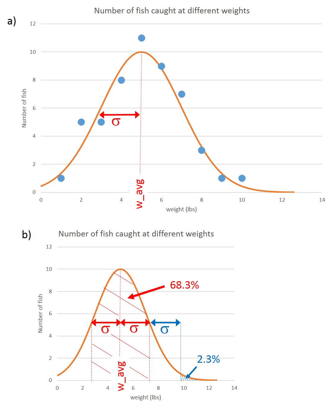
Fig. 3.1 a) Distribution of fish caught on one day (blue circles). The distribution is fitted with a bell curve (Gaussian function, orange line). The average and most probable weight is labeled w_avg while the width of the distribution is given by σ. b) from the distribution in a) we can estimate how many fish will be a lot heavier than the average weight. 68.3% of the fish will be within σ of the average (red hashed region between 3 and 7 lbs) but 2.3% will be heavier than 10 lbs, which is 2σ away from the average (blue hashed region). 0.14% of the fish will be heavier than 12 lbs, which is 3σ away from the average.
Although an air rifle is deterministic and, in principle, if we knew all the parameters (pellet shape, weight, air pressure, wind speed, barrel orientation, pressure amplitudes and locations in holding the stock, etc); we could predict very precisely where the pellet would land. However we don’t know all these parameters, so we have to accept that since the parameters vary a little bit from shot to shot, we will get a spread of pellet impacts on the target. The rifle isn’t truly shooting randomly about some central point, but since we can control/know the parameters only to a limited extent, the shots appear to randomly fluctuate around the target. This is why we shoot a series of shots (a group) to determine and improve the accuracy of our air rifles. One of the most satisfying and meditative experiences is shooting an air rifle that puts one pellet after another into the same hole at the target, also better known as “group therapy.” Conversely, one of the most frustrating experiences is shooting a rifle that sprays pellets all over the target and doesn’t respond to our best efforts to make it more accurate. But what do these groups tell us and how can we use them to assess a rifle’s accuracy?
Also, how many shots should we put in each group?
Before we start talking about pellet groups at a target, it helps to introduce one of the most fundamental ideas in statistics, the random walk. My favorite way to discuss the random walk is with a simple story. Imagine a drunken sailor who starts walking along a line. Sorry all you sailors out there, but the drunken sailor walk is a pretty standard concept in statistics! It also fits with the fishing theme that we explored at the beginning of this chapter. The sailor, let’s say Captain Haddock for you Tintin fans, has a 50% chance of stepping forward and a 50% chance of stepping backward after each step. Where will the sailor wind up after 10 steps? To answer that question we need to look at statistics. If we do this experiment over and over again, we’ll find that we get a distribution of final positions of the sailor after 10 steps. Most of the time, the sailor will be back close to his starting position after taking nearly the same number of steps forward and backward. There are lots of ways to get 5 steps forward (F) and 5 steps backward (B). For example, he could do 5 steps forward followed by 5 steps backward (FFFFBBBBB). He could alternate going forward and backward (FBFBFBFBFB). You can see that there’s lots of ways to arrange 5 Fs and 5 Bs to write the sailors stepping history. In fact there’s 252 ways to arrange 5 Fs and 5 Bs in a string of 10 steps. What the farthest the sailor could be from the starting point after 10 steps? That is simply 10 steps forward (or 10 steps backward). There’s no way he could wind up 11 steps from the starting position since he only took 10 steps. So how likely is it that the sailor winds up 10 steps in front of the starting position? Well, there is only one way to do this, with the sailor taking all 10 steps forward (FFFFFFFFF). One of the most important principles in statistics is that the more ways a certain result can be achieved, the more likely it is to happen. It turns out the probability that the sailor winds up 10 steps in front of the starting point after taking 10 steps is 1/1024=0.001, where 1 represents the number of ways the sailor can take all 10 steps forward and 1024 is just the number of all possible outcomes. There are 2*2*2*2*2*2*2*2*2*2=2 to the tenth power=2^10=1024 possible outcomes since for every step there are two possibilities and the possibilities multiply to get the total number of possibilities. We use the caret symbol ^ to indicate an exponent or “to the power of.” On the other hand, the probability that the sailor winds up back at the starting point is 252/1024=0.246, where 252 is the previously calculated number of ways to combine 5 Fs with 5 Bs and the 1024 is the total number of possible outcomes. So the sailor is 252 times more likely to wind up at the starting position than 10 steps in front of the starting position!
We can extend this random walk to two dimensions by allowing the sailor to step left or right as well as forward or backward. So for each step, there’s a 25% chance the sailor will go forward, a 25% chance he will go right, a 25% chance the he will go backward and a 25% chance he will step to the left. This is shown for 12 steps in Fig. 3.2a). This type of thought experiment can also be applied to shooting pellets at a target. I’ve coined this the “drunken marksman” problem where there’s a 25% chance that a shot will be one unit up, right, down, or left from the previous shot. As you can see in Fig. 3.2b) this is starting to look like a group of shots at a target!
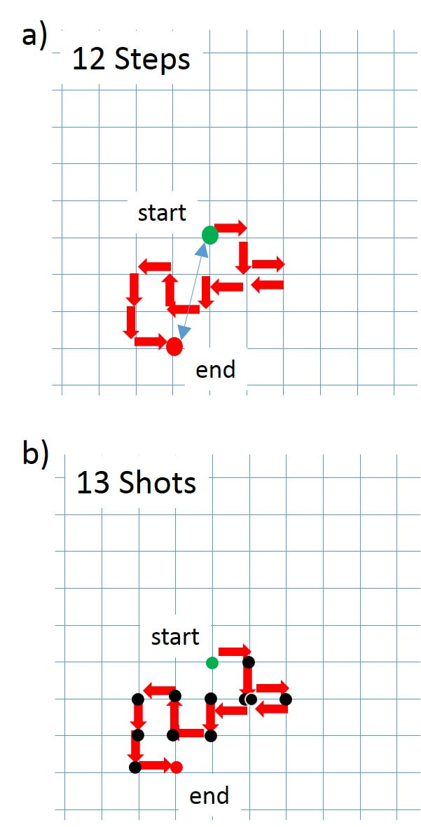
Fig. 3.2 a) Drunken sailor random walk and b) drunken marksman’s group on a target.
In order to see what kind of groups a drunken marksman would shoot, I wrote a computer program that takes random steps up, down, left or right from the previous shot. In Fig. 3.3 the program has generated twenty 5-shot groups using the random walk approach. The size of each group is characterized by the center-to-center (ctc) distance between the shots that are the farthest apart, measured from the centers of the two holes that are farthest apart on the paper. Some group are tiny, others are more stretched out. They don’t look very different from 5-shot groups that I’ve produced with my air rifles.
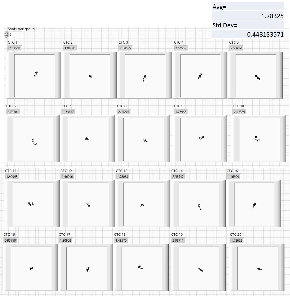
Fig. 3.3 Twenty 5-shot groups from the drunken (random walk) marksman.
In Fig. 3.4 the same program has generated ten 10-shot groups. These tend to be larger than the 5-shot groups, as there is a greater tendency to wander away from the starting point as more shots are added. Again, some groups exhibit lots or backtracking and therefore are small, whereas other groups tend to be more stretched out.
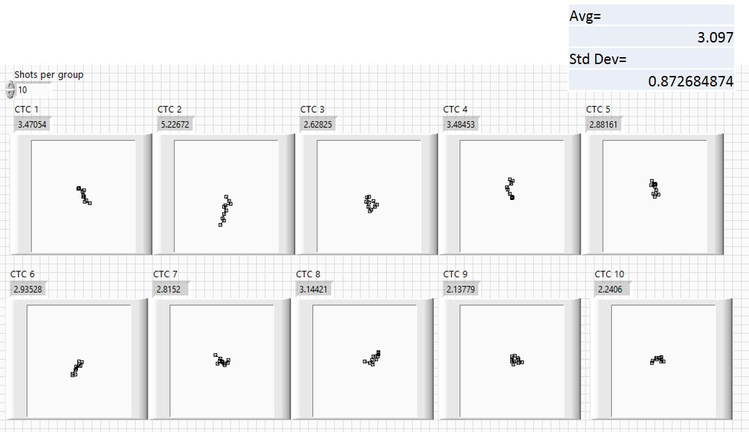
Fig. 3.4 Ten 10-shot groups from the drunken (random walk) marksman.
Finally, we look at five 20-shot random walk groups in Fig. 3.5a). These are a bit bigger, but the main difference is that they are more uniform in size. When calculating the average ctc group size, one can also obtain the standard deviation of that average, which tells us how much variation there was in the samples that produced that average value. In Fig. 3.5b) I plot the average group size and the standard deviation of the average (vertical error bars) for the 5-, 10-, and 20-shot groups that the computer created. You can see a slight increase in average size of the groups as the number of shots per group goes up. You can also see how the error bars get smaller as the number of shots per group goes up. Please note, that all these averages involve 100 shots (20 times 5 shots, 10 time 10 shots, and 5 times 20 shots). The difference between the 10- and 20-shot averages is well within the error bars.
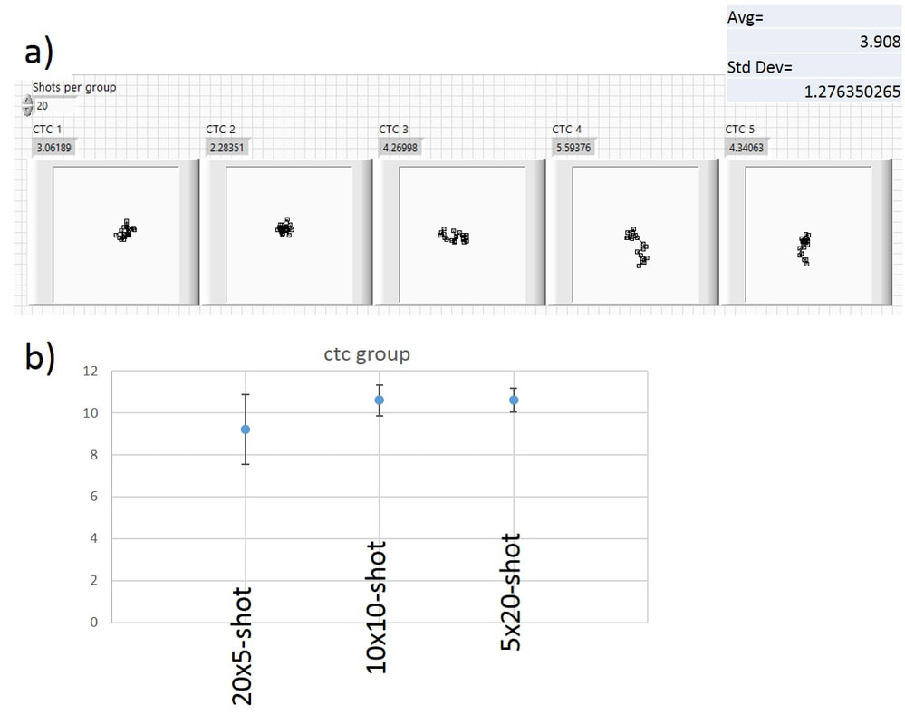
Fig. 3.5 a) Five 20-shot groups from the drunken (random walk) marksman. b) Average ctc distances with error bars for twenty 5-shot, ten 10-shot and five 20-shot groups.
So how are these groups sizes distributed? Do they make a nice bell curve? To test this, I had the computer generate 100,000 10-shot groups and looked at the distribution of group sizes. I measured the group size two ways. The first way was the ctc distance, as discussed earlier and shown in Fig. 3.6a). This is the easiest way to determine the size of real groups, where one can simply use a caliper to measure the distance between the centers of the two shots that are the farthest apart. Since I’m using a computer to generate these groups, I also can use a technique that is more commonly used for scientific data. This technique is shown in Fig. 3.6b). In this case, one finds the average position of all the shots (center of the group) and measures the distances of each shot from that center. These distance are then squared, added together, and then one takes the square root of the sum and divides by the number of shots. This is called the root-mean-square distance (RMS) and is a very good measure of how closely spaced all the shots are. The ctc distance really only looks at the two outermost shots and cannot distinguish how the rest of the shots are grouped, so the RMS distance gives a more complete picture of how well ALL the shots are grouped together. Of course, on a real target, figuring out the RMS distance would be very time consuming so we always use ctc distance, but I thought this would be a good opportunity to compare these two ways of determining group size. The RMS distance also has useful statistical meaning that is very similar to the standard deviation s that we discussed earlier. We expect that around 67% of all shots fired will be inside of a circle with a radius equal to the RMS distance. For an excellent article on characterizing group distributions at the Lapua test center, please take a look at:
https://www.snipershide.com/precision-rifle/22lr-lot-testing-at-lapuas-indoor-100m-test-facility-what-should-you-expect-in-gains/
https://www.snipershide.com/precision-rifle/22lr-lot-testing-at-lapuas-indoor-100m-test-facility-what-should-you-expect-in-gains/
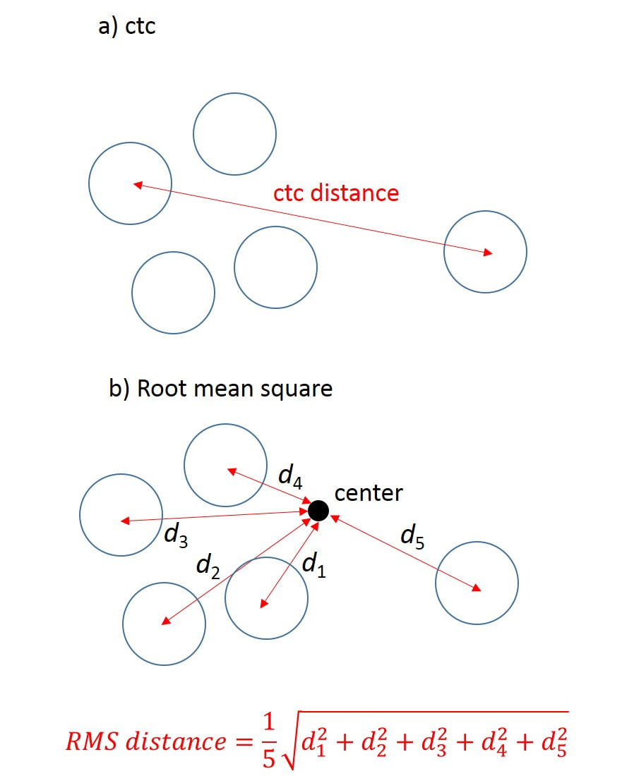
Fig. 3.6 Determining the size of a group using a) the ctc distance and b) the root mean square (RMS) distance.
Figure 3.7 shows the distribution (the number of groups at different group sizes) of ctc and RMS group sizes for 10-shot groups. Both distributions are roughly shaped like bell curves, although they are a little asymmetric. As expected, the ctc distribution is shifted to bigger distances since it only looks at the outermost shots compared to the RMS, which also includes shots that are close to each other in the group size average. The RMS distribution is also narrower, which makes sense since it is averaging over all the shots in the group while the ctc is only looking at the outermost two shots. More shots/samples tend to result in better and more reliable averages with smaller standard deviations. I fitted both the ctc and RMS distributions with Gaussian functions to obtain the average values and the standard deviations of those averages. The standard deviation characterizes the width of the distribution and is equivalent to the σ that I introduced in Fig. 3.1.
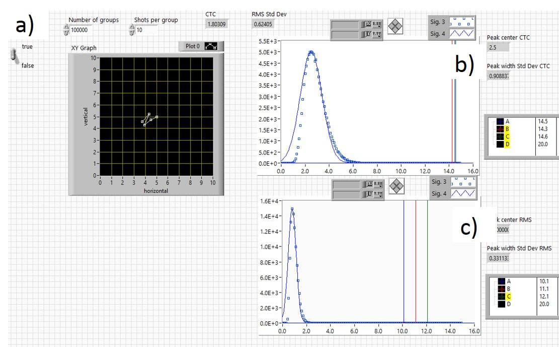
Fig. 3.7 Distribution for 10-shot groups using the drunken marksman (random walk) method. a) typical group, b) distribution of ctc and c) RMS distances for 100,000 10-shot groups.
A common question people have when testing the accuracy of a rifle is how many shots to put in each group and how many groups to fire. My program allows us to explore how group size scales with the number of shots in each group and gives insight in how to test the accuracy of a rifle. In Fig. 3.8 I plot the average ctc and RMS distance as a function of the number of shots in the group. I did this by generating 100,000 groups for each group shot count and fitting the distributions with a Gaussian to get the average ctc and RMS distances (like I did for 10-shot groups in Fig. 3.7). For a purely random system, one would expect the group size D to grow like the square root of N, where N is the number of shots in the group (or steps in a random walk). So if you double the number of shots in a group, the group size should grow by a factor of the square root of 2, which is 1.41. We can also write the square root of 2 as 2^0.5, which means “2 to the power of one half” In Fig. 3.8, I plotted the average ctc and RMS distances as functions of the number of shots in a group (N) on a log-log plot By taking the log of both the horizontal and vertical axes (log(N^0.5) vs log(D)) one can get the power of N from the slope of the line. For example, a function that goes like N^2 would have slope of 2 on the log-log plot. Also note that the square root of N corresponds to N^0.5, so if D goes like N^0.5 the slope of that function would be 0.5 on a log-log plot. I also plotted the function N^0.5 (square root of N). As you can see, all the curves in Fig. 3.8 are straight lines with pretty much the same slope, corresponding to D being proportional to N^0.5, which is exactly what we expected!
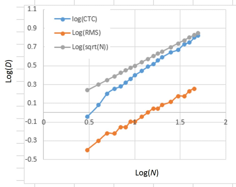
Fig. 3.8 The average ctc and RMS distances D as a function of the number of shots N in a group on a log-log plot. Also plotted is log(N^0.5), which is how we expect the average ctc and RMS distances to scale with N for a normal distribution.
Although the random walk is a good place to start, I’m not sure that it’s the best way to characterize the randomness in the point of impact (POI) of an air rifle. In my air rifles, the POI tends to fluctuate about some central point and not on the previous shot, which is how we did the random marksman thought experiment. If the air rifle’s barrel pivot bolt is getting progressively looser, then one might expect a POI to shift like a random walk, where each new POI is based on the previous POI. The same walking behavior may happen as the piston seal warms up and the friction between the seal and the compression chamber increases, gradually decreasing the muzzle velocity. In this case, the POI will walk and each new POI will fluctuate about the previous POI as the muzzle velocity steadily decreases. So if you see a drifting POI, the random walk may be the right model to analyze the groups. However, in most cases, the rifle returns pretty much to the same condition for each shot and the POI fluctuates about a fixed center, not one that gets reset to the previous POI. To model this, we just have the POI fluctuate about a fixed center rather than from the previous POI. A simple example of this is to imagine flipping a coin before each shot, as shown in Fig. 3.9a) where a head (H) means the shot lands on the left half of the target and a tail (T) means the shot lands on the right half of the target. Let’s say one makes five coin tosses and gets HHTHT, which would mean that three shots were sent to the left and two went to the right. Although it’s unlikely that one tosses five heads in a row, this will happen once in a while (with a probability of 1 in 32) and it doesn’t mean that this is special coin! The same is / could be true for a rifle that places all five shots in the same hole once in a while! One can extend this to two dimensions by using two coins, one for the horizontal direction (Coin A), like before, and a new one for the vertical direction (Coin B), as shown in Fig. 3.9b). Let’s have heads for Coin B mean the shot will go to the upper half and tails mean it will go to the lower half of the target. Again, one flips both coins before the shot, and the result of the tosses determines where the shot will go. For example, if Coin A is heads and Coin B is tails, the shot will go to the lower left quadrant. The shots are randomly distributed over four quadrants at the target. One can divide up the target into smaller pieces by using two six-sided dice, one for the horizontal direction (Die A) and one for the vertical direction (Die B), as shown in Fig. 3.9c). Now there is an equal chance for the shot to wind up in any one of the 36 squares. If Die A is a 1 and Die B is a 3, the shot will be in the first column, three rows down.
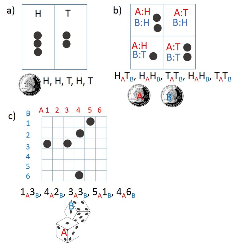
Fig. 3.9 a) single coin flip POI, two coin flip POI, and c) two dice roll POI. The results of the flip/roll randomly determine the POI for each shot.
For the computer modeling, I divided the target into a 10x10 grid and picked random numbers between 1 and 10 for both the vertical and horizontal directions for each shot. We can imagine rolling two 10-sided die to generate each POI, so I’ll call this the two-dice roll method. The first number (first die roll) decides the column of the POI and the second number (second die roll) decides the row. In Fig. 3.10, I generated twenty 5-shot groups using this technique. Although it’s equally likely that the POI for each shot would land in any one of the 100 squares at the target, one can get some pretty small groups, like the group in the lower right corner (circled in red) with a ctc of 6.4. This group is about a factor of two smaller than the group circled in the top row with a ctc of 12.0. These completely random groups are at the heart of the challenge in using a single 5-shot group to prove the accuracy of a rifle!
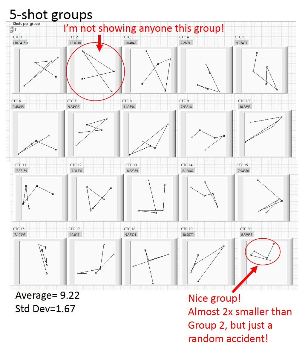
Fig. 3.10 5-shot groups generated by the two-dice roll method. Although the groups are completely random, some are a lot smaller than others, as shown by red circles!
Now let’s take a look at groups with more shots. Figure 3.11 shows ten 10-shot groups that were generated by the program. The groups are bigger (with average ctc of 10.6 compared to 9.2) and the sizes are more uniform (standard deviation of only 0.74 compared to 1.67) than the 5-shot groups.
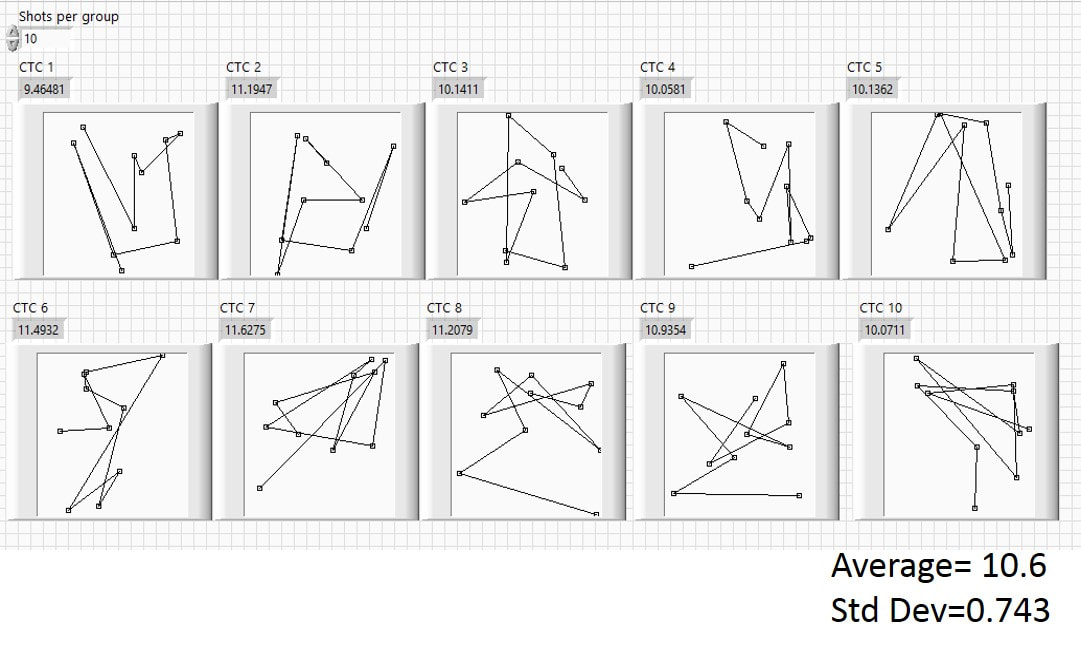
Fig. 3.11 10-shot groups generated by two-dice roll.
Going to five 20-shot groups doesn’t change things much compared to the 10-shot groups. Figure 3.12a) shows five 20-shot groups that were generated by the program. The average size (10.6) is the same and the standard deviation (0.56) is only slightly smaller than what we got for the 10-shot groups. In Fig. 3.11b) I plot the average group size and the standard deviation (vertical error bars) of the average for the 5-, 10-, and 20-shot groups that the computer created using the two-dice method. It’s very similar to the results obtained with the random walk method. You can see a slight increase in average size of the groups as the number of shots per group goes up. You can also see how the error bars get smaller as the number of shots per group goes up. Please note, that all these averages involve 100 shots (20 times 5 shots, 10 time 10 shots, and 5 times 20 shots). In this case, the difference between the 10- and 20-shots averages is even smaller compared to the random walk method and is well within the error bars.
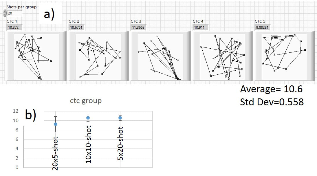
Fig. 3.12 a) Five 20-shot groups generated by two-dice roll. The groups look very similar to each other. b) Average ctc distances with error bars for twenty 5-shot, ten 10-shot and five 20-shot groups.
So how do the group size distributions look with the two-dice roll method? Just as I had done with the random walk method, I had the computer generate 100,000 3-shot groups using the two-dice roll method and looked at the distribution of group sizes. Again, I looked at both ctc and RMS to characterize group size. Figure 3.13 shows the distribution of ctc and RMS group sizes for 3-shot groups. A typical 3-shot group is shown in Fig. 3.13a). Figures 3.13 b) and c) show the distributions of the ctc and RMS distances, respectively. The distributions are fitted well by Gaussians. We can use the probability properties of Gaussian distributions that we introduced in the fishing example at the beginning of this chapter to analyze the 3-shot distributions. The red rectangle in Fig. 3.13b) shows that 16% of the groups have ctc distances smaller than 4.9, which is just over half of the average value (7.1). That means that one out of every six 3-shot groups has a ctc that is far below the average value. So if one picks the “best” group out of five or six groups, one could well be picking a group that is accidentally small! The blue rectangle in Fig. 3.13b) shows that 2% of the groups have ctc distances smaller than 2.7, which shows that once in a while one can get really tiny groups by accident, just like catching that 12 lb haddock! Figure 3.12c) looks at the RMS group sizes.
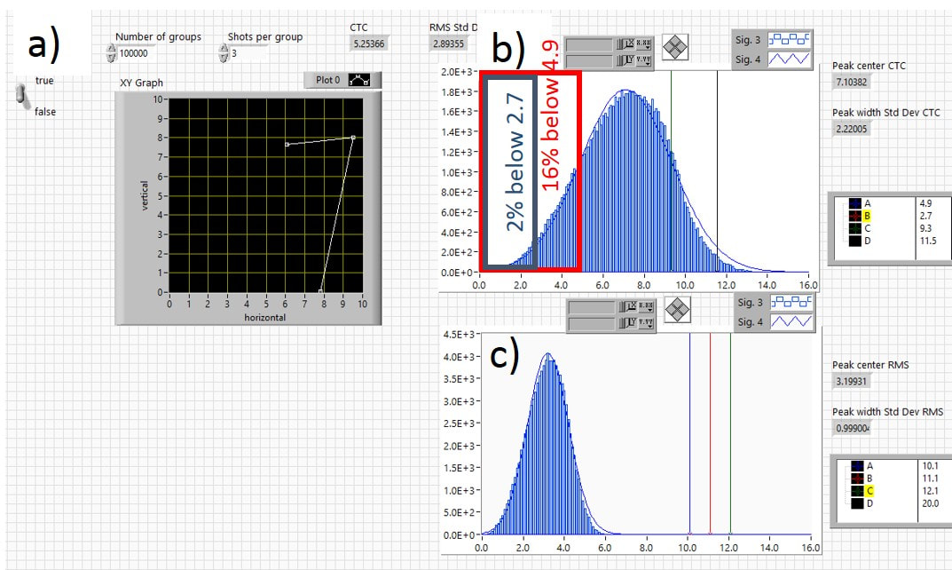
Fig. 3.13 Distribution for 3-shot groups using two-dice roll. a) typical group, b) distribution of ctc and c) RMS distances for 100,000 3-shot groups.
Now let’s look at groups with more shots in them. Figure 3.14 looks at the distribution of 100,000 5-shot groups using the two-dice roll method. A typical 5-shot group is shown in Fig. 3.14a). Figures 3.14 b) and c) show the distributions of the ctc and RMS distances, respectively. As with the 3-shot distributions, the 5-shot distributions are fitted well by Gaussians. The red rectangle in Fig. 3.14b) shows that 16% of the groups have ctc distances smaller than 7.4, which is much closer to the average value of 9 compared to the 3-shot distribution.
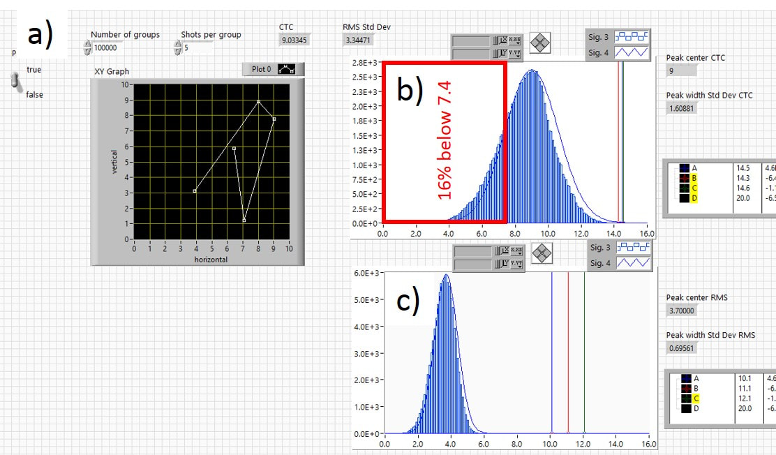
Fig. 3.14 Distribution for 5-shot groups using two-dice roll. a) typical group, b) distribution of ctc and c) RMS distances for 100,000 5-shot groups.
Figure 3.15 looks at the distribution of 100,000 10-shot groups using the two-dice roll method. A typical 10-shot group is shown in Fig. 3.15a). Figures 3.15 b) and c) show the distributions of the ctc and RMS distances, respectively. The 10-shot distribution has a larger average and is much narrower than the 3- and 5-shot distributions. Now the chance of getting a dramatically smaller than average group is greatly reduced.
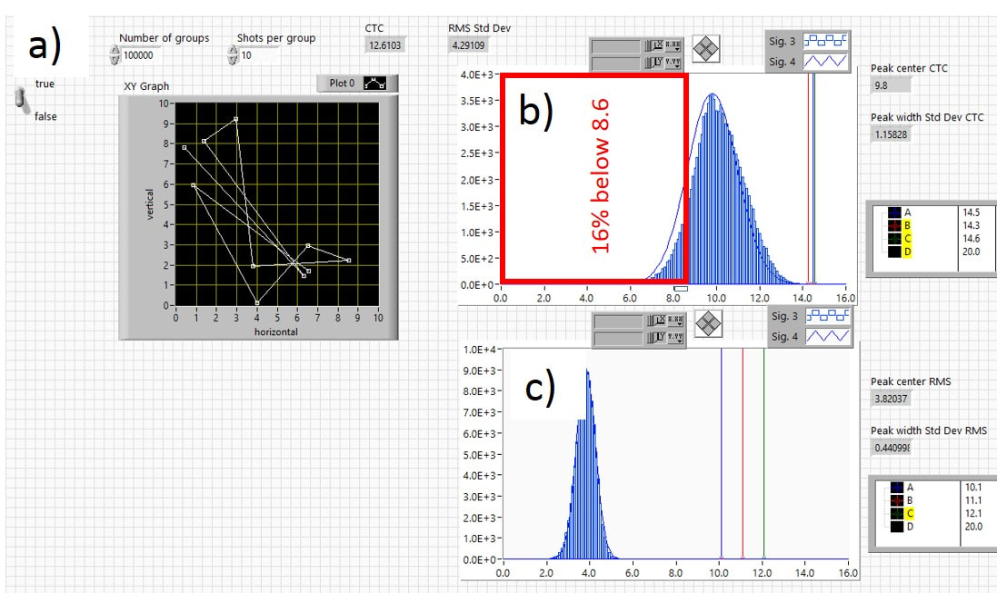
Fig. 3.15 Distribution for 10-shot groups using two-dice roll. a) typical group, b) distribution of ctc and c) RMS distances for 100,000 10-shot groups.
Finally, we look at the distribution 100,000 20-shot groups using the two-dice roll method. A typical 20-shot group is shown in Fig. 3.16a). Now we can see that the group size is starting to be limited by the 10x10 grid target that we defined in the two-dice roll calculation. By definition, all shots will fall in the 10x10 grid, so no matter how many shots are fired, the group size cannot grow beyond this square. This may seem like an arbitrary limit on group size, but it is not unrealistic. This group size limit prompted me to coin a term that I call the point of impact envelope (POIE). This is probably a well-known concept, but I couldn’t find it described anywhere, so please let me know if I should reference someone here. I think that every rifle has a POIE in which it will keep all its shots unless something disastrous happens. For example, there may be some side-to-side play in the barrel of a break-barrel springer, but as long as one doesn't loosen the barrel tension screw or hit the barrel to one side with a hammer, the range of possible orientations of the barrel will always be within a certain range and the horizontal spreading of shots due to barrel orientation will be the same whether 10 or 1,000 or 10,000 shots are taken (of course, there may be effects of wear after thousands of shots). This is in contrast to the random walk/drunken sailor problem, where a sailor randomly takes steps left or right, each with a 50% probability. In that case, the spread of final distances away from the starting point grows without any limits as more steps are taken, albeit only growing as the square root of the number of steps since the randomized stepping tends to cancel large excursions to the right or left.
Figures 3.16 b) and c) show the distributions of the ctc and RMS distances, respectively, for 20-shot groups. Now the distributions are fitted really well by Gaussian functions! The 20-shot distributions have slightly larger averages and are slightly narrower than the 10-shot distributions. Clearly, adding more shots after 10 is not making much of a difference!
Figures 3.16 b) and c) show the distributions of the ctc and RMS distances, respectively, for 20-shot groups. Now the distributions are fitted really well by Gaussian functions! The 20-shot distributions have slightly larger averages and are slightly narrower than the 10-shot distributions. Clearly, adding more shots after 10 is not making much of a difference!
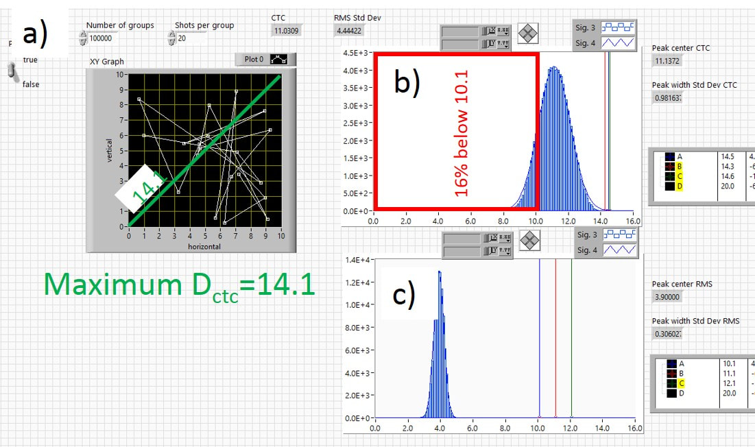
Fig. 3.16 Distribution for 20-shot groups using two-dice roll. a) typical group, b) distribution of ctc and c) RMS distances for 100,000 20-shot groups. The distribution now looks very “normal” and is fitted very well by a Guassian function!
Finally, we look at the scaling of the average group size with the number of shots in the group using the two-dice roll method in Fig. 3.17. Figure 3.17a) plots the average (over 100,000 groups) ctc and RMS distance D as functions of the number of shots in the groups N. Clearly the group size is saturating towards a constant value as N increases. Since all the shots must be within the 10x10 square, the largest distance between shots is the diagonal across the square, which has a value of 14 and is indicated by the horizontal red line in Fig. 3.17a). Since we expect D to go as a power p of N (D=C[N]^p, where C is just a constant) if we plot log(D) vs log(N) we should get a straight line where the slope of that line is just p, as shown in the equations in Fig. 3.17b). For small N with log(N)<0.6, the slope is pretty close to 0.5, which is what we expected and obtained from the random walk. This makes sense because for small N, the groups aren’t really bumping up against the boundaries of the 10x10 target grid. However, when log(N)>0.6, the slope is more like 0.2 or 0.1, which means that D=C[N]^0.2 or D=C[N]^0.1. In Fig. 2.4 in Ch. 2 we looked at the scaling of average ctc with the N in real rifles shooting real groups. For both the LGU and FWB 124 shooting 5-, 10-, and 20-shot groups, the group sizes scaled as N^p with p being significantly smaller than the expected 0.5. For the FWB 124, p was 0.36, and for the LGU it was around 0.29.
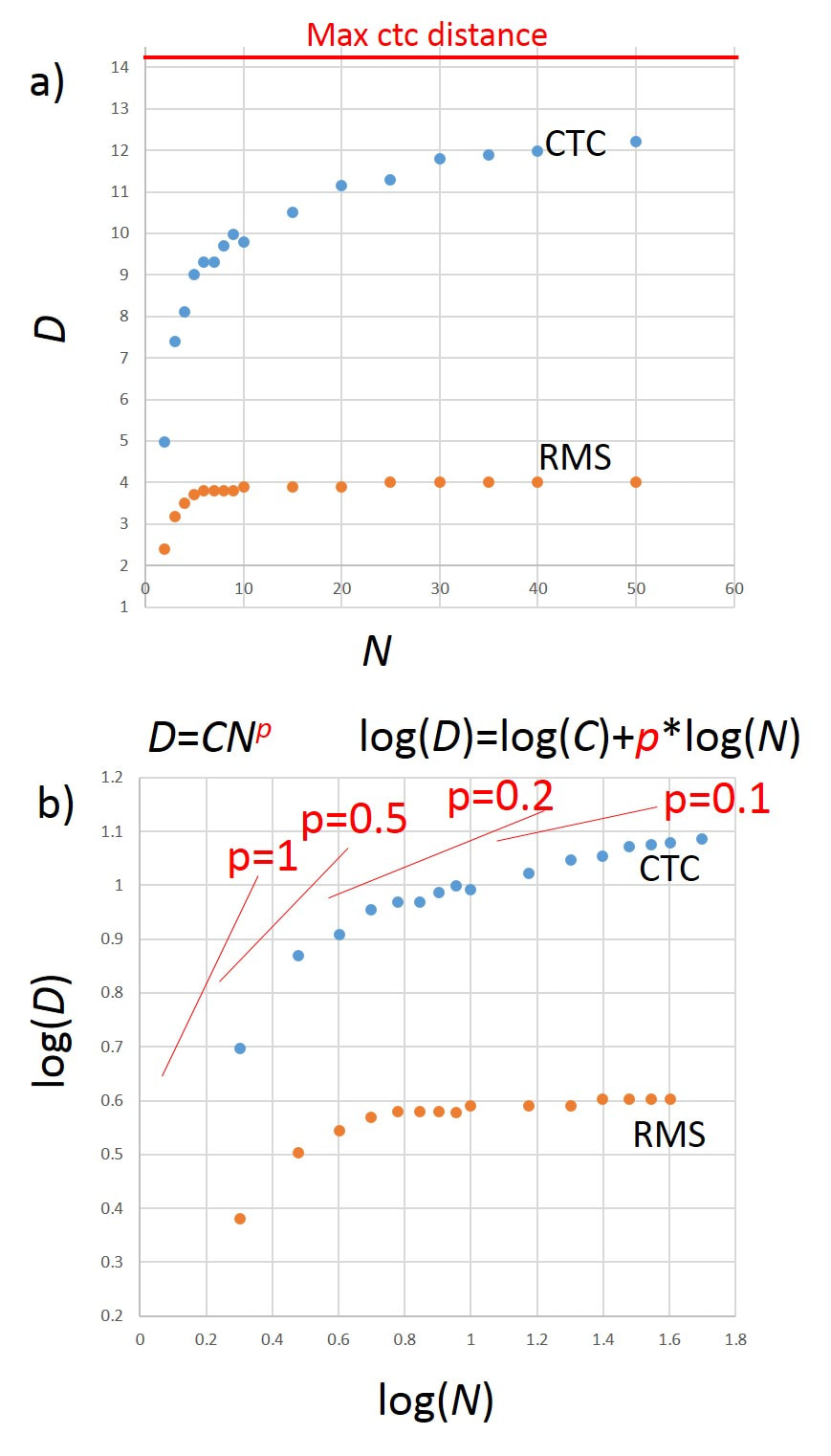
Fig. 3.17 a) Average ctc and RMS distances D as functions of the number of shots N in group. b) Average ctc and RMS distances as functions of the number of shots in group on a log-log plot, so the slope gives the power of N that the data follow. For example, slope p=0.5 corresponds to N^0.5 behavior, which is expected for a normal distribution.
Before summing up, I’d like to thank our brave readers for slogging through lots of technical ideas and equations to get to the end of this chapter! I hope that you didn’t find this chapter too complex and confusing, and even if you did, I hope that you will consider the following conclusions:
1. We can model groups shot from rifles two basic ways: either with the random walk (drunken marksman) or with the two-dice roll methods. In both cases, POI fluctuates randomly, but in the random walk we start each new shot from where the previous one hit and in the two-dice roll we always go back to the same central position and randomly jump to the next POI from there. Both methods produce groups that look like real groups shot from air rifles. The random walk group sizes scale as N^0.5 (N is the number of shots in the group), as one would expect from the basic properties of normal distributions, while the two-dice roll group sizes scale more like N^0.2 or N^0.1. The real groups shot from my LGU and FWB 124 go as like N^0.29 and N^0.36, respectively, and are somewhere in between these two scaling results. We can also expect the group size to never exceed the point of impact envelope (POIE), so we know the normal distribution scaling of N^0.5 cannot hold as N gets really big.
2. A single 3-, or 5-, or even 10-shot group doesn’t mean much. We can accidentally get very small groups, especially if we don’t have many shots in the group. So how many shots in a group and how many groups are needed to test the accuracy of a rifle? Part of the answer depends on how consistent your group sizes are. For example, I just shot my LGU at 10 yards and every 5-shot group was a single hole about the size of a pellet. There’s not much point shooting lots of groups with many shots in each group for that situations. At 20 yards in Chapter 2 we saw bigger fluctuations from group to group, especially when the number of shots per group was smaller, so we decided that ten 10-shot groups was more than enough. However, more data is always better. I’ve been scanning in all the targets of all my rifles for the past five years. I’ve even saved and have now scanned targets that were shot in the late 1990s. I have over 300 Powerpoint slides of targets (probably over 4000 groups!) and notes for my FWB 124 alone. Having such a digital record really helps me improve and troubleshoot these rifles.
3. After looking at the range of group sizes that we can get due to purely random fluctuations, we should not just pick the best group that we shot and use that to characterize the accuracy of a rifle. If one is shooting outdoors in the wind and one can see shots affected by the wind, then it may make sense to weigh groups more heavily where the wind was calmer than groups where one could call bad shots due to wind. This would also be true if shooting from a less stable position and one group may have been better since the shooter was able to control sway better. In those cases, the best group makes sense, but again consistency over many shots is really the key to accuracy, not just a cherry-picked group! On the other hand, in my indoor 20 yd accuracy tests, there were no external factors that could hurt accuracy. There was no wind, I used a high power scope and stable rest, and the light triggers allowed most external factors to be removed. I think any variations in the POI in Ch. 2 were purely due to fluctuations in the rifles themselves. In that case, picking the best group would really mean just picking the group where the fluctuations happened to cancel each other out a bit better. Looking at a single 5-shot group (or even worse, a single 3-shot group!) is a bit like dividing a 5 km footrace into 10 m sections. If I (a middle-aged guy who hates to exercise) ran a 5 km race against a top athlete, there could be some 10 m sections of the race where I was faster, perhaps where I sprinted like crazy before collapsing from exhaustion! On the other hand, the top athlete would post consistently short times for each 10m section of the race and would clearly beat me to the finish line. So comparing my best time for a 10m section of the race with the top athlete’s best time for a 10m section would simply not reflect reality! A single group, gives us only a very brief glimpse of a rifle’s race to accuracy. Testing and achieving high accuracy is really more like a marathon, where we look for consistency over long times and under different conditions.
 RSS Feed